Compute persistence relative to a boundary
Suppose a segment joins two endpoints. Its edge has a nonzero boundary, so it does not represent an ordinary homology class in degree one. If we agree to count chains supported on the endpoints as zero, that same edge becomes a cycle. This is the idea of relative homology: for a space $K$ and a subcomplex $A$, we work with chains in $K$ modulo chains in $A$. A chain is a linear combination of cells, and it is a cycle when its boundary is zero. We will compute the interval of the relative edge class and then recover its endpoint boundary through the connecting map.
The input is a finite filtered complex and a selection of its cells. We use rational grades and coefficients in $\mathbb F_3$, the field of integers modulo three, so that the two endpoint signs remain distinguishable.
import TamerOp as OP
using SparseArrays: sparse
using TamerOp.CoreModules: F3

segment = OP.GradedComplex(
    [[10, 20], [30]],
    [sparse(reshape([-1, 1], 2, 1))],
    [(0//1,), (0//1,), (1//1,)],
)
pair = OP.filtered_pair(segment, [[1, 2], Int[]]; field=F3())
diagram = OP.persistence_diagram(pair)
OP.essential_births(diagram; dim=1)    # [1//1]
Here the vertices have labels 10 and 20, and the edge has label 30, with boundary [20] - [10]. Both vertices enter $K$ at parameter zero, and the edge enters at one. The inner vectors in filtered_pair select positions within each dimension: [1, 2] selects both vertices, while Int[] selects no edges. These positions are distinct from the labels 10, 20 and 30. With no separate grades supplied, the selected vertices enter $A$ at the same time as they enter $K$.
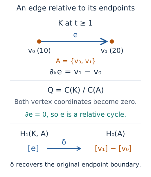
The edge survives when we set the endpoint chains equal to zero. Its relative boundary is therefore zero, although its original boundary in $K$ is $v_1-v_0$. This schematic shows the chain calculation at any parameter at least one; it does not draw a new geometric realization of the quotient.
The relative class has interval $[1,\infty)$: once the edge appears, nothing in this filtered pair can make it a boundary or remove it from the quotient. There is no relative $H_0$ because both vertices already belong to $A$.
To recover the edge's original boundary, we need homology bases at a scale where it exists. These queries live in TamerOp.Advanced, which we import as OA:
import TamerOp.Advanced as OA

h = OA.relative_homology(pair; scale=1//1)
OA.dimensions(h)                       # [0, 1]
maps = OA.relative_maps(h; dim=1)
maps.connecting                      # 2 × 1: [2; 1] over F₃
The dimensions are those of relative homology in degrees zero and one. The connecting map takes the relative edge class to its boundary class in $H_0(A)$, namely [20] - [10]. Over $\mathbb F_3$, minus one is two, which explains the first entry of the column. Its rows use the chosen basis of $H_0(A)$, and its column uses the chosen basis of $H_1(K,A)$. These bases belong to this scale; they do not name individual barcode intervals.
In a larger example, inspect the representatives and the cell order before interpreting a matrix:
OA.basis(h; dim=1)                   # The edge represents the relative class.
c = OA.relative_complex(h)
OA.relative_cells(c; dim=1)          # ambient position 1, cell ID 30
OA.relative_boundary(c; dim=1)       # a 0 × 1 zero matrix
The last matrix has no rows because the quotient has no vertices. Its one column is the edge, whose relative boundary is zero.
Let the subcomplex change later
A selected cell can enter $A$ after it has entered $K$. Keep the same ambient segment, but let the first vertex enter $A$ at two, the second at three, and the edge at four:
changing = OP.filtered_pair(segment, [[1, 2], [1]];
    grades=[[2//1, 3//1], [4//1]], field=F3())
d = OP.persistence_diagram(changing)
OP.finite_intervals(d; dim=0)          # [(0//1, 1//1), (0//1, 2//1)]
OP.finite_intervals(d; dim=1)          # [(3//1, 4//1)]
Until parameter two, $A$ is empty, so the relative calculation agrees with the absolute one: two components appear at zero and merge at one. When the first vertex enters $A$ at two, the remaining component class becomes zero. The edge still has the other vertex as its relative boundary, so it is not yet a relative cycle. At three both endpoints belong to $A$, making the edge a cycle; at four the edge itself enters $A$, and its class becomes zero.
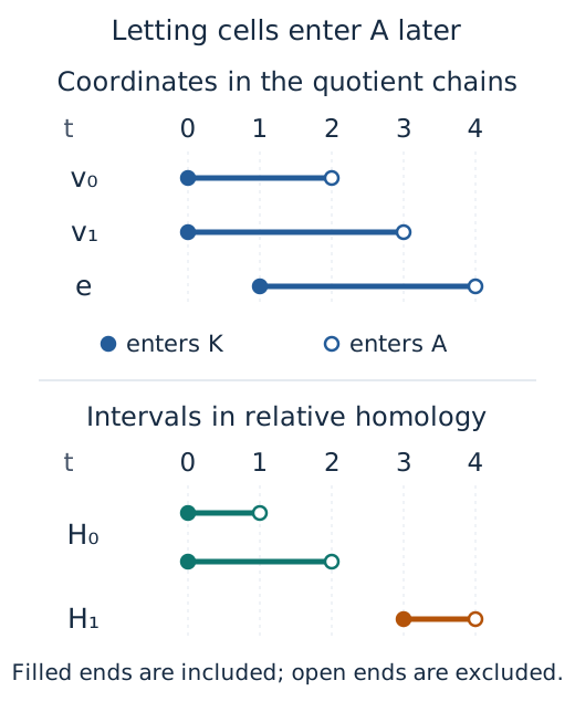
The upper rows show when each cell is available as a quotient coordinate. The lower rows show the resulting homology intervals. Having an edge coordinate at one does not yet give a relative class: its boundary vanishes only when the second endpoint enters $A$ at three.
Choose a parameter in the schematic below to follow that calculation one event at a time. The two drawings show the cells of $K_t$ and $A_t$; the table records the remaining quotient coordinates and their boundary over $\mathbb F_3$. In particular, compare one, two and three: the edge is present throughout, while its boundary loses one endpoint and then the other. The homology dimensions count the classes after taking those boundaries into account.
Solid cells are present. Faint dashed cells show what has not entered yet.
| Vertex coordinates in C₀(Kₜ,Aₜ) | None |
|---|---|
| Edge coordinates in C₁(Kₜ,Aₜ) | e |
| Boundary of e in the quotient | 0 (a 0 × 1 matrix) |
| Dimension of H₀(Kₜ,Aₜ) | 0 |
| Dimension of H₁(Kₜ,Aₜ) | 1 |
At three both endpoints belong to A. Their quotient coordinates are zero, so the edge is a cycle. There are no cells of dimension two to fill it, giving one relative class.
This is an authored schematic of the exact calculation in the recipe. The table describes quotient chain coordinates, without drawing a geometric quotient space.
We can inspect the map that ends this interval directly:
before = OA.relative_homology(changing; scale=3//1)
after = OA.relative_homology(changing; scale=4//1)
OA.relative_structure_map(before, after; dim=1)  # 0 × 1
The source has the edge class and the target is zero, so the matrix has one column and no rows. Deleting all cells that will eventually enter $A$ would erase this interval before it had a chance to appear.
An empty selection, [Int[], Int[]], recovers absolute persistence. Selecting all cells with their inherited grades gives zero relative homology. In either case, the selection must still form a subcomplex: selecting this edge requires both endpoints, and the edge cannot enter $A$ before either endpoint does. The constructor checks these conditions over the selected field.
The pair reference specifies input and map conventions. To see how the computation accommodates coordinates that disappear from the quotient, follow the implementation account. The ordinary persistence guide describes the interval queries and diagram analysis available for this result.