Constructing modules without a filtration
Download the executed notebook · Build and environment record
Sometimes the spaces and maps are the data we want to start with. Perhaps we have a small example in mind, or want to see what happens when one matrix changes. We can give that diagram to TamerOp directly and use the same queries and algebraic operations available for modules obtained from a filtration.
We will work over the rational numbers, starting with four one-dimensional spaces arranged in a diamond. Following a vector around its two sides will tell us whether our matrices define a module. We will then enlarge one space and construct a second example from indicator regions, whose boundaries determine where the module is nonzero.
You need Julia, TamerOp and CairoMakie, together with matrix multiplication and the meaning of a structure map. We use OP for the main interface and A = OP.Advanced for detailed matrix queries and editor controls. The editor reference gives the accepted inputs and limits.
import TamerOp as OP
using CairoMakie
A = OP.Advanced
TamerOp.AdvancedEnter the finite diagram
The four vertices have relations $1<2<4$ and $1<3<4$, with 2 and 3 incomparable. At each vertex we put a copy of $\mathbb Q$. This vector space is the module's stalk there. Initially each arrow carries the identity matrix, so a scalar starting at 1 arrives unchanged at 4 along either route.
The order matrix records order[i,j] = true when $i\leq j$, including the diagonal and the composite relation $1\leq4$. We supply structure matrices only for covers, comparable pairs with no intervening vertex. Composing these matrices gives the maps for longer relations.
order = Bool[1 1 1 1;
             0 1 0 1;
             0 0 1 1;
             0 0 0 1]
cover_maps = Dict((1, 2) => [1;;], (1, 3) => [1;;],
                  (2, 4) => [1;;], (3, 4) => [1;;])
Dict{Tuple{Int64, Int64}, Matrix{Int64}} with 4 entries:
(2, 4) => [1;;]
(1, 2) => [1;;]
(1, 3) => [1;;]
(3, 4) => [1;;]editor = OP.module_editor(; order, dimensions=[1, 1, 1, 1], maps=cover_maps)
@assert A.check_module_editor(editor).valid
OP.describe(editor)(kind = :module_editor, valid = true, input_kind = :module, field = TamerOp.CoreModules.CoeffFields.QQField(), selection = (vertex = 1, edge = (1, 2), revision = 0), revision = 0, closed = false, updating = false, undo_count = 0, redo_count = 0, history_limit = 32, listener_count = 0, listener_errors = (), limits = (max_vertices = 32, max_dimension = 32, max_entries = 20000))The editor keeps the entered data as a draft and checks whether they define a module. The first view draws the covers as a Hasse diagram, with arrows pointing upward in the order. Their positions help us see the diamond; the horizontal distances do not describe a parameter space. As throughout the guide, a matrix has one row for each target coordinate and one column for each source coordinate.
initial_diamond = OP.editor_object(editor)
OP.visualize(A.inspection_snapshot(editor))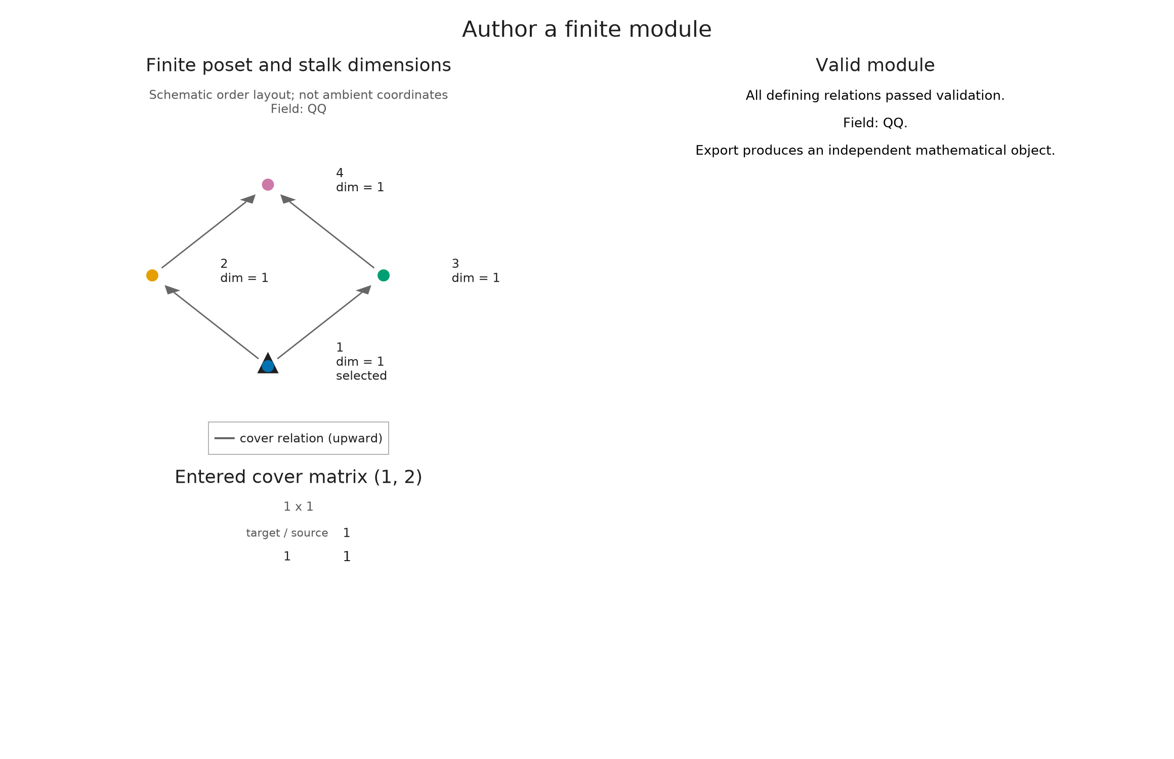
Make the two routes disagree
Suppose we change the map from 3 to 4 to multiplication by 2. A scalar $a$ now arrives at 4 as $a$ along the left route and $2a$ along the right. In a module over a poset, the relation $1\leq4$ has a single structure map, so these answers must agree for every $a$.
This is the compatibility to predict before running the edit: each individual matrix still has the right shape, but the four matrices no longer describe a module.
OP.edit_module!(editor; map=((3, 4), [2;;]))
report = A.check_module_editor(editor)
@assert !report.valid
report.issues
1-element Vector{String}:
"Paths 1 -> 2 -> 4 and 1 -> 3 -> 4 have different composites."witness = report.witness
@assert witness.first_path == [1, 2, 4]
@assert witness.second_path == [1, 3, 4]
@assert witness.first_composite == [1;;]
@assert witness.second_composite == [2;;]
(first=witness.first_composite, second=witness.second_composite)(first = Rational{BigInt}[1;;], second = Rational{BigInt}[2;;])The report retains both paths and their products, $[1]$ and $[2]$, so we can locate the disagreement in the draft. The draft remains available for correction. Trying to obtain a module with OP.editor_object(editor) or to export Julia construction code at this point would fail, because there is no map for $1\leq4$ compatible with both routes.
incompatible_diamond = OP.visual_state(A.inspection_snapshot(editor))
OP.visualize(A.inspection_snapshot(editor))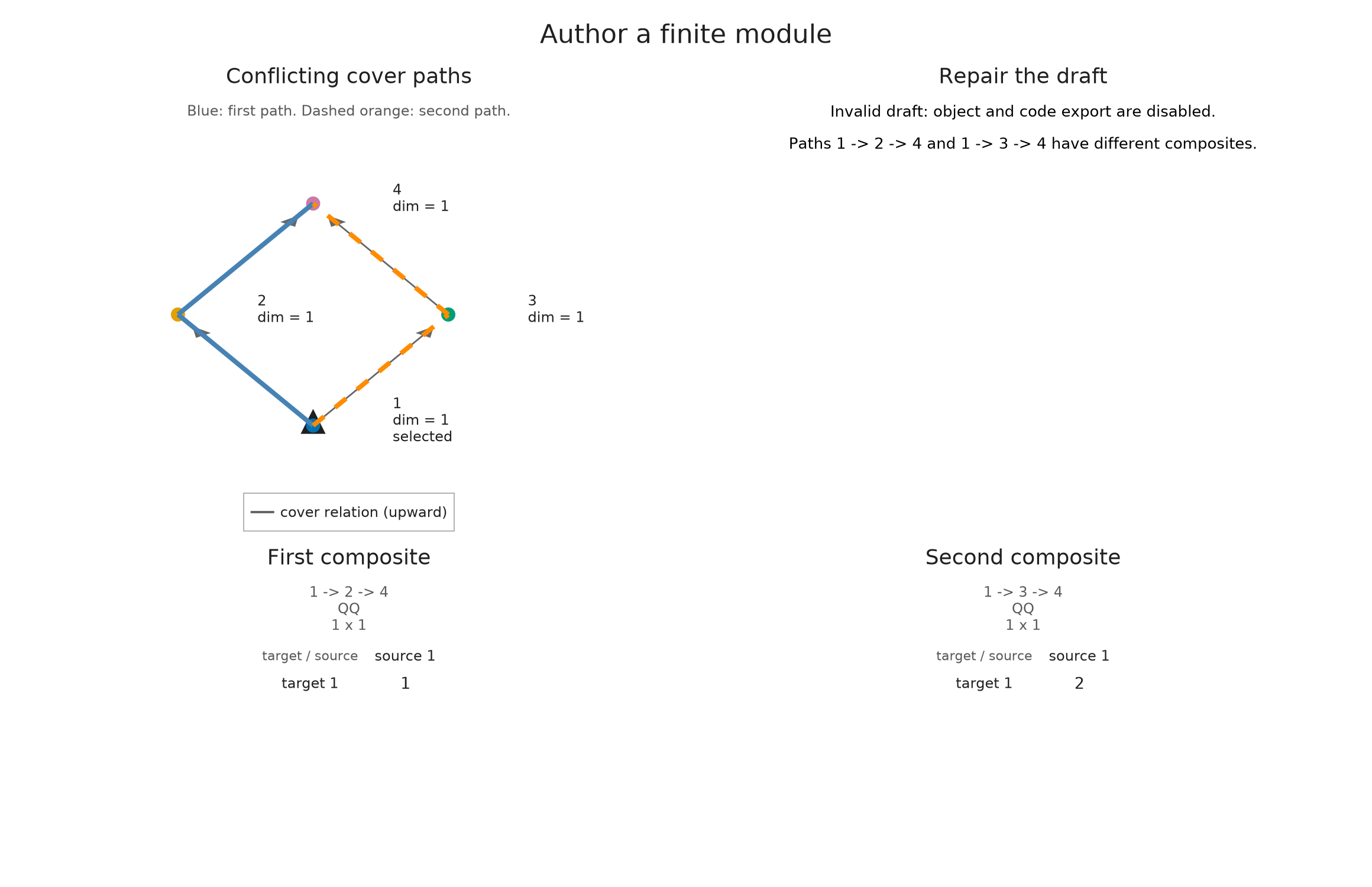
Repair, then change the target space
Undo returns to the commuting diamond. We can now replace its terminal space by $\mathbb Q^2$ and send a scalar $a$ to $(a,2a)$. Both incoming maps must be columns with two rows. Supplying both columns makes the new dimensions and the compatibility visible in the input; the editor does not resize a matrix to guess the intended map.
A.undo_module_edit!(editor)
@assert A.check_module_editor(editor).valid
larger_maps = copy(cover_maps)
larger_maps[(2, 4)] = reshape([1, 2], 2, 1)
larger_maps[(3, 4)] = reshape([1, 2], 2, 1)
OP.edit_module!(editor; dimensions=[1, 1, 1, 2], maps=larger_maps)
A.select_inspection!(editor; vertex=4, edge=(3, 4))
ModuleEditorSession(module, valid=true, revision=4, closed=false)M = OP.editor_object(editor)
@assert OP.dimensions(M).stalks == [1, 1, 1, 2]
@assert A.structure_map(M; source=1, target=4) == reshape([1, 2], 2, 1)
A.structure_map(M; source=1, target=4)2×1 Matrix{Rational{BigInt}}:
1
2OP.visualize(A.inspection_snapshot(editor))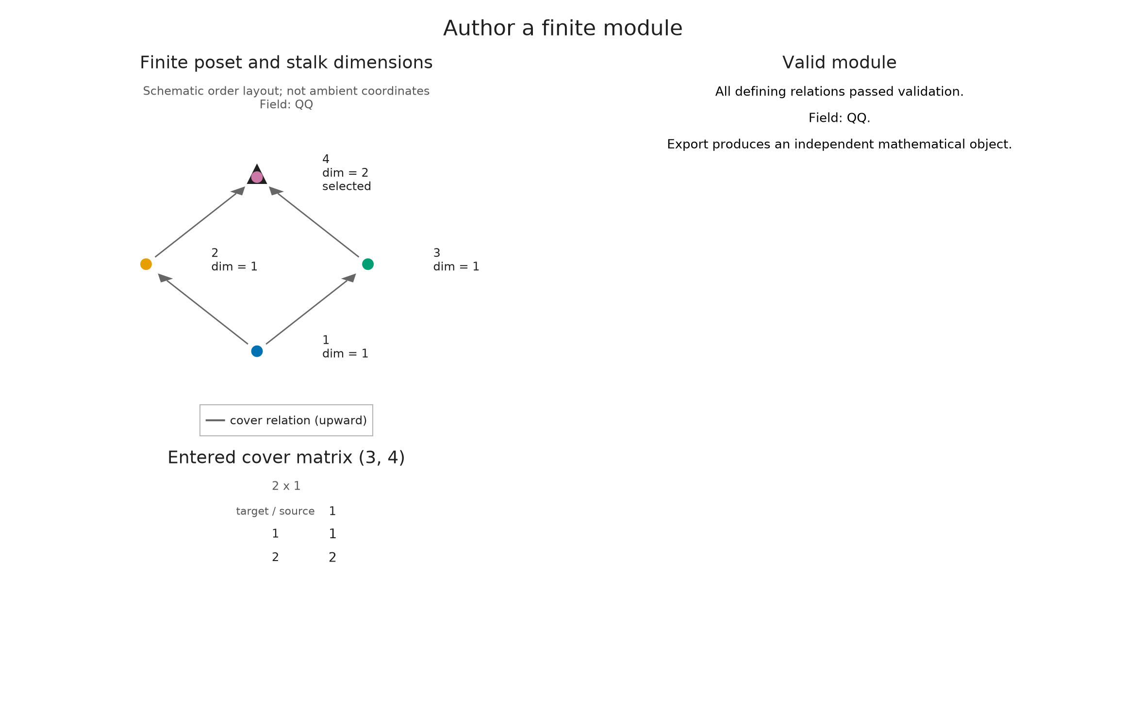
The returned M is a module on this finite poset, with its own spaces and maps. Subsequent edits to the draft leave it unchanged. The composite matrix just displayed sends $a\in M(1)$ to $(a,2a)\in M(4)$, which gives us a concrete map to use in the spaces and maps guide.
A diagram on four labels is already a mathematical input. To interpret it over a lattice or continuous parameter space, we would additionally need a classifier, an order preserving map assigning an original parameter to a finite label. The drawing does not supply that map.
Follow the changes to the diamond
The prepared comparison returns to the three diagrams. In the commuting diamond, the map from 1 to 4 is $[1]$. The incompatible draft shows its two paths separately, with products $[1]$ and $[2]$. After enlarging the target, the map from 1 to 4 is the column $(1,2)^{\mathsf T}$. Follow the matrix shape together with the dimension at vertex 4.
An indicator presentation is another input
We can describe a module by specifying where its generating coordinates are allowed to occur. On the chain $1<2<3$, let $U=\{2,3\}$ be an upset: once a vertex belongs to $U$, every larger vertex does too. Let $D=\{1,2\}$ be a downset, closed in the opposite direction. The indicator module of either set has a copy of $\mathbb Q$ on the set, zero outside, and identity maps between comparable vertices in the set.
A coefficient $1$ gives a map from the indicator of $U$ to the indicator of $D$. Its image is one-dimensional where both are active, which is just vertex 2. Here the editable matrix supplies coefficients between indicators. It serves a different purpose from the cover matrices of our diamond. This description by an image is called a fringe presentation; indicator presentations develops the construction for several generators.
presentation = OP.module_editor(; order=Bool[1 1 1; 0 1 1; 0 0 1],
    upsets=[[2, 3]], downsets=[[1, 2]], matrix=[1;;])
A.select_inspection!(presentation; vertex=2)
H = OP.editor_object(presentation)
@assert OP.dimensions(H).fibers == [0, 1, 0]
OP.visualize(A.inspection_snapshot(presentation))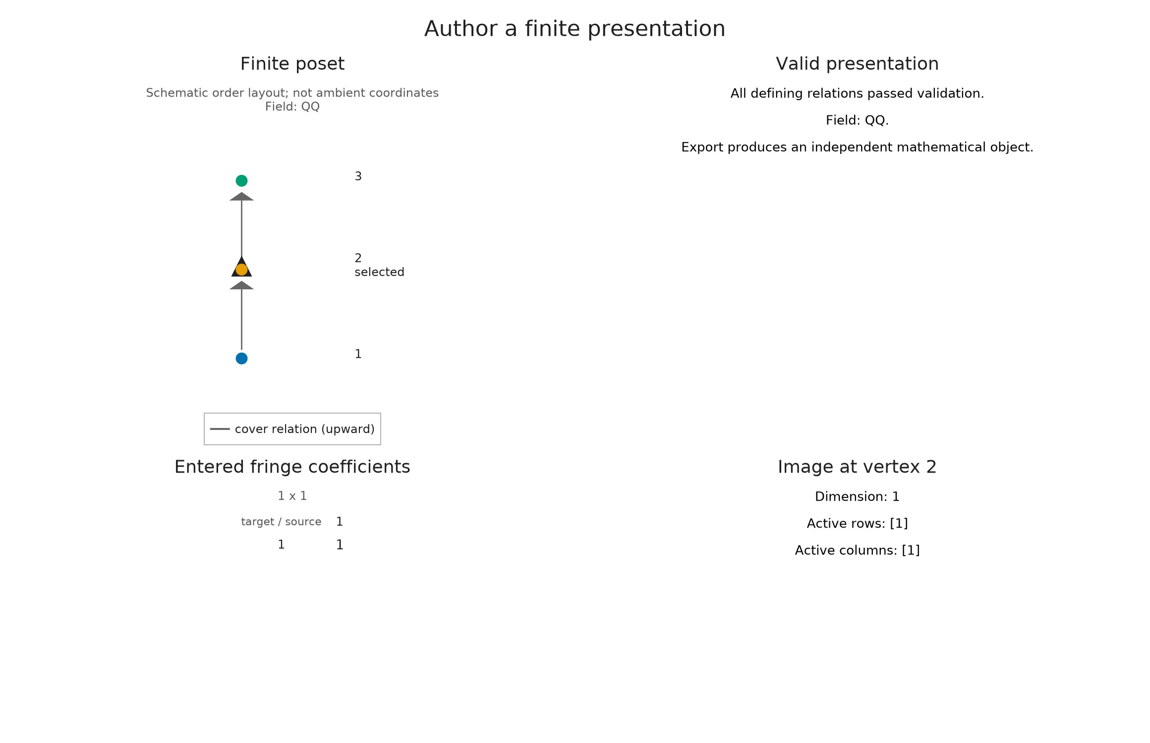
With coefficient zero, the image becomes zero at every vertex while the two chosen indicator supports stay in the presentation. This lets us see how the coefficient matrix affects the represented module even when the regions are fixed. The closure conditions on the supports matter as well: the editor rejects an entered upset or downset that fails its condition instead of adding vertices to it.
OP.edit_module!(presentation; matrix=[0;;])
@assert OP.dimensions(OP.editor_object(presentation)).fibers == [0, 0, 0]
OP.visualize(A.inspection_snapshot(presentation))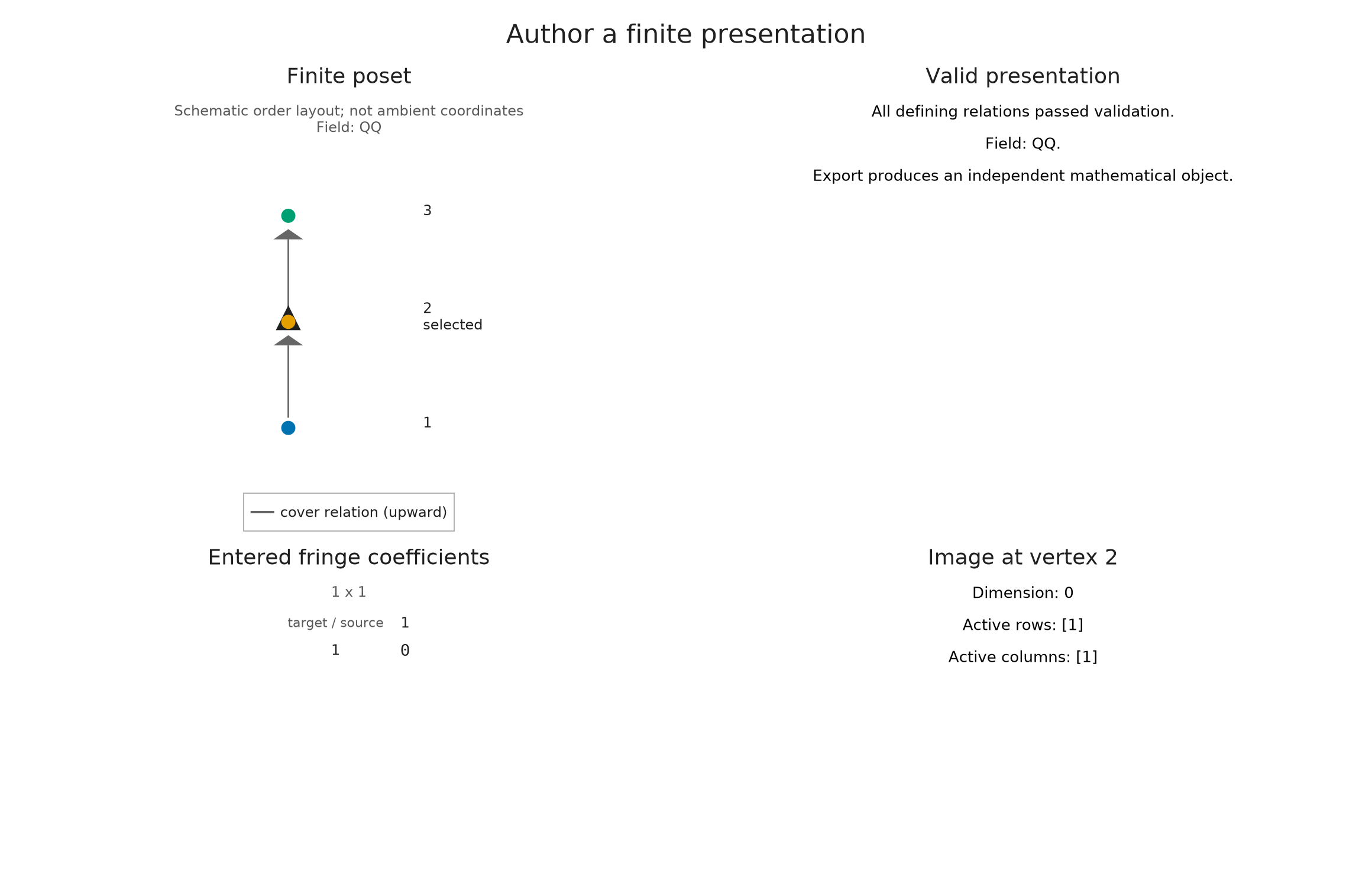
A.close_inspection!(presentation)
ModuleEditorSession(presentation, valid=true, revision=2, closed=true)Give the presentation a parameter space
The same idea applies to regions of $\mathbb R^2$ ordered coordinatewise. Take $U=[0,\infty)^2$ and $D=(-\infty,0]\times(-\infty,2]$, again with coefficient 1. Their intersection is the closed segment $\{0\}\times[0,2]$. A point on that segment carries $\mathbb Q$, even though the segment has zero area.
BoxUpset specifies the lower corner of an unbounded upset and BoxDownset the upper corner of an unbounded downset. encode constructs a finite module and its classifier from these regions. Here backend=:pl_backend selects the specialized construction for boxes, and field specifies rational linear algebra. These integer corner coordinates are exactly representable in the box format.
options = A.EncodingOptions(; backend=:pl_backend,
    poset_kind=:signature, field=OP.CoreModules.QQField())
segment = OP.encode([A.BoxUpset([0, 0])], [A.BoxDownset([0, 2])],
    OP.QQ[1;;], options)
segment_module = OP.encoding_module(segment)
segment_classifier = OP.encoding_map(segment)
OP.describe(segment)
(kind = :encoding_result, poset_type = TamerOp.ZnEncoding.SignaturePoset{1, 1}, module_type = TamerOp.Modules.PModule{Rational{BigInt}, TamerOp.CoreModules.CoeffFields.QQField, Matrix{Rational{BigInt}}, TamerOp.ZnEncoding.SignaturePoset{1, 1}}, encoding_map_type = TamerOp.EncodingCore.CompiledEncoding{TamerOp.PLBackend.PLEncodingMapBoxes{2, 1, 1}, TamerOp.ZnEncoding.SignaturePoset{1, 1}, Nothing, Nothing, TamerOp.CoreModules.EncodingCache}, compiled = true, backend = :pl_backend, has_cohomology = true, has_presentation = true, module_dims = [0, 0, 1, 0], materialized = true, provenance = (category = :finite_poset_representations, base_poset = SignaturePoset(regions=4, flats=1, injectives=1), field = TamerOp.CoreModules.CoeffFields.QQField(), degree = nothing, degree_convention = :not_applicable, encoding = (map_type = TamerOp.EncodingCore.CompiledEncoding{TamerOp.PLBackend.PLEncodingMapBoxes{2, 1, 1}, TamerOp.ZnEncoding.SignaturePoset{1, 1}, Nothing, Nothing, TamerOp.CoreModules.EncodingCache}, backend = :pl_backend), window = :unrestricted, orientation = :coordinatewise, construction = (requested = :presentation_encoding, effective = :presentation_encoding, substitution = :none), discretization = (kind = :finite_encoding, filtration_values = :not_resampled), approximation = (construction = :none_requested, geometry = :backend_numerical_contract, strict_eps = nothing, effective_strict_eps = nothing, feasibility = :not_applicable), backend = (requested = :pl_backend, effective = :pl_backend), ambient_identification = :not_asserted, refinement = :single_encoding))To recover the answer at an original parameter, first locate its label and then query the finite module. The endpoints $(0,0)$ and $(0,2)$ are included, and the map between them must be an isomorphism of one-dimensional spaces. A point just to the right of the segment has a represented zero stalk. We ask the classifier for each label rather than assuming the numbering chosen by the encoder.
bottom = A.locate(segment_classifier, (0, 0))
top = A.locate(segment_classifier, (0, 2))
off_segment = A.locate(segment_classifier, (1, 1))
segment_map = A.structure_map(segment_module; source=bottom, target=top)
@assert A.dim_at(segment_module, bottom) == A.dim_at(segment_module, top) == 1
@assert A.dim_at(segment_module, off_segment) == 0
@assert segment_map == OP.QQ[1;;]
segment_map
1×1 Matrix{Rational{BigInt}}:
 1
OP.visualize(segment; kind=:module_inspector,
parameter_pair=((0, 0), (0, 2)), box=([-1.0, -1.0], [1.0, 3.0]))
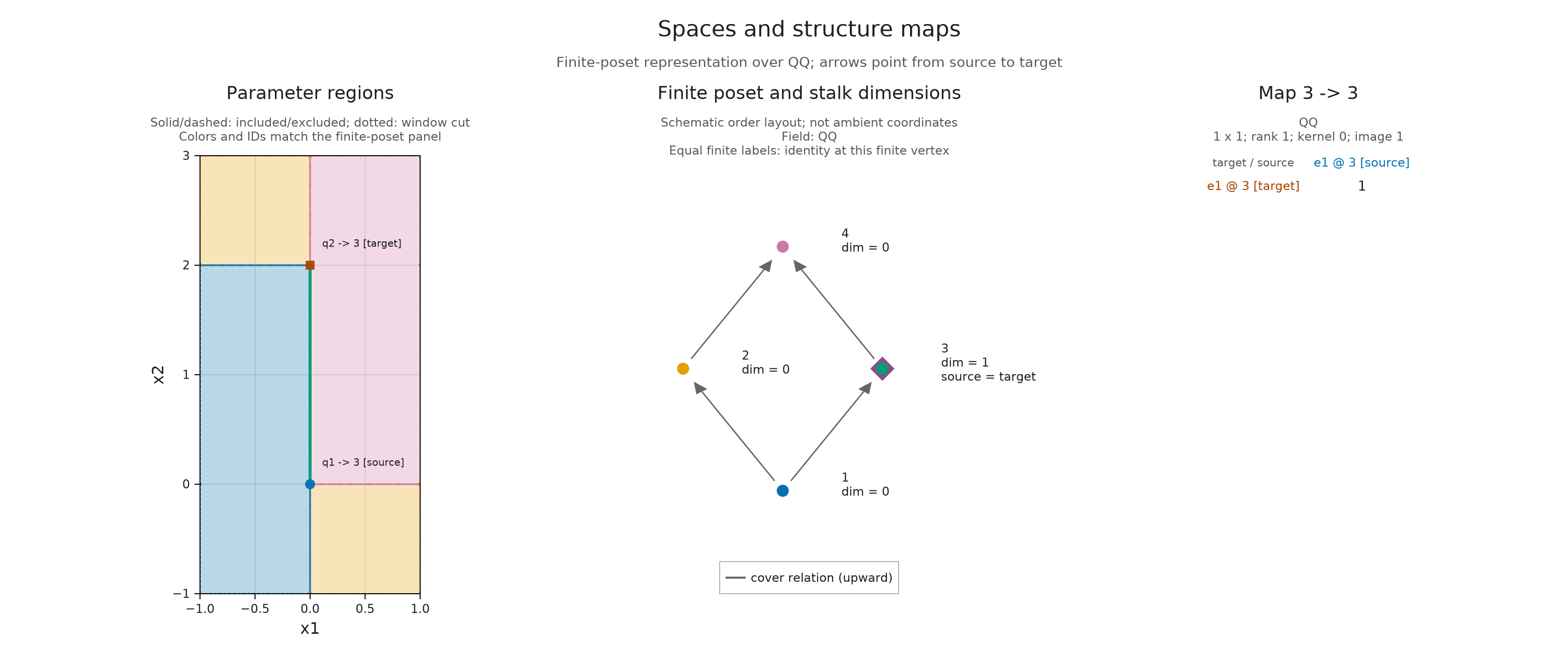
If we make the upper corner $(0,0)$ as well, the support shrinks to a single closed point. The classifier must retain this point separately from its zero neighbors for the same reason it retained the segment.
point_module = OP.encode([A.BoxUpset([0, 0])], [A.BoxDownset([0, 0])],
    OP.QQ[1;;], options)
point_classifier = OP.encoding_map(point_module)
origin = A.locate(point_classifier, (0, 0))
neighbor = A.locate(point_classifier, (0, 1))
@assert OP.dimensions(point_module)[origin] == 1
@assert OP.dimensions(point_module)[neighbor] == 0
(origin_dimension=OP.dimensions(point_module)[origin],
 neighbor_dimension=OP.dimensions(point_module)[neighbor])
(origin_dimension = 1, neighbor_dimension = 0)The choice of representation follows the supplied mathematics. A finite diagram starts with its labels and all required cover maps. A lattice presentation records generators and relations at integer grades. Geometric presentations supply regions in a real parameter space; boxes suffice for coordinate inequalities, while sloped boundaries require polyhedral regions. The input guide works through a sloped strip using the general polyhedral route.
For box encodings, OP.encoding_representatives(segment) returns exact rational points belonging to the classifier regions. They are witnesses for the stored box thresholds, which use floating point coordinates; they do not restore precision lost before those thresholds were supplied. The box encoding account explains boundary cells and these representatives. A lattice classifier has a different domain, so rounding a real point to an integer label is not an interchangeable interpretation of this segment.
representatives = OP.encoding_representatives(segment)
@assert all(A.locate(segment_classifier, x) == q for (q, x) in enumerate(representatives))
representatives
4-element Vector{Tuple{Rational{BigInt}, Rational{BigInt}}}:
 (-1, -1)
 (1, -1)
 (0, 1)
 (1, 1)
Edit through a live viewer
With WGLMakie loaded, OP.visualize(editor; backend=:wglmakie) opens controls for editing this draft in a Julia session. The matrix and dimension controls let you repeat the changes above, and the viewer displays a failed path when the draft stops defining a module. Generating Julia code requires a valid draft; preparing a saved draft can retain an invalid one for later diagnosis.
The live inspection guide explains session controls and display support distinguishes a standalone Julia-backed browser window from an embedded notebook viewer.
Optional: prepare the diamond comparison
The initial module and the failed draft were retained before the editor changed them. We can now place their drawings alongside the final module. The failed draft contributes its two composite matrices and the paths that produced them; the ordinary editor utilities are unnecessary for this comparison.
@assert A.structure_map(initial_diamond; source=1, target=4) == OP.QQ[1;;]
@assert A.structure_map(M; source=1, target=4) == reshape(OP.QQ[1,2],2,1)
failed_snapshot = A.inspection_snapshot(incompatible_diamond)
failed_paths = OP.compose_visuals((
    paths=OP.visual_panel(failed_snapshot; panel=1),
    first_route=OP.visual_panel(failed_snapshot; panel=3),
    second_route=OP.visual_panel(failed_snapshot; panel=4));
    columns=3, title="The two paths give different maps", subtitle="Rational coefficients; the entered diagram does not define a module.")
diamond_views = (;
    var"Commuting diamond"=A.visual_spec(initial_diamond; kind=:module_inspector, pair=(1,4)),
    var"Incompatible paths"=failed_paths,
    var"Two dimensional target"=A.visual_spec(M; kind=:module_inspector, pair=(1,4)))
presentation_directory = joinpath("tamerop_outputs", "presentations")
mkpath(presentation_directory)
OP.save_visual_session(joinpath(presentation_directory, "diamond.html"), diamond_views;
    selected=Symbol("Commuting diamond"), size=(1400,650),
    title="Follow a scalar from vertex 1 to vertex 4",
    caption="Both paths must give the same map over Q. Compare the identity, the incompatible draft and the common column into a two dimensional target.");
A.close_inspection!(editor)
ModuleEditorSession(module, valid=true, revision=4, closed=true)These constructions now lead to modules whose spaces and maps we can investigate. The spaces and maps guide follows that investigation through selected stalks, matrices and ranks. If you already have a finite diagram and want the construction procedure at hand, the short recipe keeps it in one place.