From selected images to submodules and quotients
A vector can disappear under a structure map while another vector in the same space survives. If we want the submodule generated by a particular selection, we therefore need to follow its coordinates through the maps. The dimensions of the ambient spaces alone cannot tell us what was generated.
This account follows the computation from selected columns to their image spaces, the induced submodule maps and the quotient projection. The usage guide develops the example of two overlapping square supports; the module reference gives the accepted shapes and coefficient fields. Throughout, a stalk means the vector space at one vertex of the finite poset. The matrices below use columns for source coordinates and rows for target coordinates.
Propagate columns before constructing a new module
Let $M$ be a module on a finite poset $P$, choose a vertex $p$, and place $s$ selected vectors from $M(p)$ in the columns of a matrix $B$. At each vertex $q\geq p$, the columns we want are
\[Y_q=M(p\leq q)B.\]
The vertices $q\geq p$ form the upper ideal of $p$. Outside this set there is no forward structure map from the source, and the stored image is nothing. Inside it, a zero matrix means that the selected vectors have zero image. Its row and column counts still record the target dimension and the number of supplied vectors.
propagate first checks the module's storage, then visits successors along covers, relations with no intervening vertex. The first path to a vertex supplies its image columns. When another incoming cover reaches a vertex already visited, the algorithm compares its product with the stored columns and raises an error if they disagree. Multiplying the cover matrices by $B$ and its subsequent images avoids constructing entire composite matrices for a selection of only a few vectors.
Over an exact field, agreement on every applicable cover establishes path independence for the selected columns. Indeed, induction along any path shows that its partial products equal the stored columns at the vertices it visits. The ambient diagram is still required to be a module: these checks concern the selected vectors and do not establish compatibility on all other vectors. The result retains the supplied columns, including dependent ones, and computes their image rank at each visited vertex.
For example, take $M(u)=\mathbb Q^2$, $M(v)=\mathbb Q$, and cover matrix $M_{uv}=[0\;1]$. Selecting $e_1$ gives zero at $v$; selecting $e_2$ or $e_1+e_2$ gives the scalar 1. All three selections see the same rank-one ambient map, yet they answer different questions about individual vectors. The prepared vector comparison lets us follow these choices through the two square supports and compare their generated spaces away from the selected target too.
The generated spaces are
\[N(q)=\begin{cases}\operatorname{im}Y_q,&p\leq q,\\0,&\text{otherwise}.\end{cases}\]
They are closed under structure maps because $M(q\leq r)Y_q=Y_r$ whenever $p\leq q\leq r$; maps starting at a zero generated space satisfy closure as well. Every submodule containing the original columns contains all their images, proving that this construction is the smallest such submodule.
Use the existing image engine
The propagation result stops at image columns and ranks. On an explicit generated_submodule call, the library constructs a module $F$ with $s$ coordinates at every vertex above $p$, identity maps between these spaces, and zero spaces elsewhere. Each coordinate is a copy of the principal projective at $p$. Giving a morphism from this module to $M$ amounts to choosing a vector at $p$ and following it forward; for $s$ copies the choices are exactly the columns of $B$.
The resulting morphism $F\to M$ has component $Y_q$ at $q\geq p$. Calling image_submodule on it lets the general image construction supply both the image spaces and their maps. At each vertex, that construction selects independent columns $I_q$ spanning the image. For a cover $u<v$, its induced matrix $N_{uv}$ is obtained from
\[I_vN_{uv}=M_{uv}I_u.\]
The right side takes each image basis vector at $u$ through the ambient map. Closure puts the resulting columns in the image space at $v$, and independence of the columns of $I_v$ makes their coordinates unique. The matrices $I_q$ are therefore the components of the inclusion $N\hookrightarrow M$.
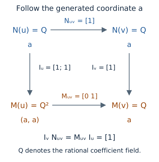
This schematic uses the selection $e_1+e_2$ in the example above. The induced map is $[1]$ because $[0\;1](1,1)^{\mathsf T}=1$. Its value follows from the inclusions and the ambient map; equal image dimensions alone would not specify it.
The same image construction serves a general module morphism. The kernel construction instead chooses bases of the component nullspaces and recovers its induced maps by the corresponding inclusion equation. Both use the shared rank and coordinate routines described in Exact rational coordinates. Prime fields retain exact arithmetic too. With RealField, ranks and equation comparisons depend on the configured tolerances, so numerical agreement does not prove exact path independence. check_propagation checks the retained source columns, image ranks and every applicable cover equation under the field's conventions.
Remove the generated submodule
quotient_with_projection calls the general cokernel construction on the inclusion. At each vertex, it chooses a matrix $Q_q$ whose kernel is the included image space and whose rows give coordinates in the quotient. Vectors have the same quotient coordinates precisely when their difference belongs to the image. The quotient's cover matrix $\overline M_{uv}$ is determined by
\[\overline M_{uv}Q_u=Q_vM_{uv}.\]
In our example, we can choose $Q_u=[-1\;1]$: it kills $(1,1)^{\mathsf T}$ and maps $\mathbb Q^2$ onto a one-dimensional space. At $v$, the image fills the ambient space, so the quotient is zero and $Q_v$ has zero rows. The quotient cover map is consequently the unique map $\mathbb Q\to0$. These are illustrative coordinate choices; the constructor may return a different basis for the same quotient.
The equation $Q_qI_q=0$ records that the projection annihilates the included space, while the displayed cover equation records compatibility with the module maps. The construction also gives $\dim(M/N)(q)=\dim M(q)-\dim N(q)$, so its projection has exactly the required kernel. Matrices with zero rows or columns participate in these same equations.
A quotient need not be realizable by a complementary submodule inside $M$. For the chain $\mathbb Q\xrightarrow{1}\mathbb Q$, selecting a vector at the second vertex generates $0\to\mathbb Q$. Its quotient has dimensions $(1,0)$, but a complement with those dimensions would fail to be preserved by the ambient identity map.
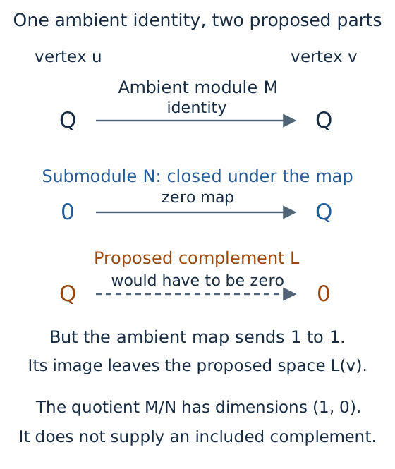
Choosing complementary vector spaces separately at the vertices does not ensure that the module maps preserve them. This example explains why forming a generated submodule and quotient does not certify a direct sum decomposition.
The image, kernel and quotient constructions also supply other categorical operations. For maps $f:X\to Z$ and $g:Y\to Z$, a pullback consists of pairs $(x,y)$ with $f(x)=g(y)$, so it is computed as the kernel of $[f\;-g]:X\oplus Y\to Z$. Dually, a pushout identifies the two images of each vector in a common source by taking a cokernel of the corresponding signed map. Keeping the inclusions and projections makes these constructions usable for further maps, beyond knowing their dimensions.
Coordinates, source cycles and reuse
Suppose invertible matrices $C_q$ convert old stalk coordinates to new ones. The stored map from $p$ to $q$ then becomes $C_qM_{pq}C_p^{-1}$, and the selected source columns become $C_pB$. Their propagated images are $C_qY_q$, so image ranks and nonzero support agree. The new inclusion represents the same subobject under this specified module isomorphism. Replacing a basis of the selected subspace by another basis also preserves its generated subobject, although individual column matrices change.
For a homology module, a source cell query can express a propagated column in a supplied target homology basis of retained cycles. It checks the cycle equations and that the supplied classes form a basis modulo the active boundaries. The identification of this ordered basis with the module's coordinates is supplied explicitly by the caller and recorded. The account of source representatives explains these chain correspondences.
A propagation result retains the ambient module, the selected columns and their images; an encoding input retains its classifier as well. With $s$ columns, the image matrices contain $s\sum_{q\geq p}\dim M(q)$ coefficients, in addition to the retained input objects. Cover multiplication depends on the matrix dimensions and storage. Storage validation examines the ambient module, the propagation checks each applicable cover on its selected columns, and rank calculations can account for much of the work when many columns are supplied. Rational coefficient sizes affect arithmetic costs beyond these counts of entries.
Reading an image or summary returns copies of the stored data. Constructing a submodule additionally allocates the projective source, image bases and induced cover maps; forming a quotient constructs another set of coordinates and maps. Rendering requests neither construction implicitly. The viewer's finite graph budget limits the number of drawn vertices, while matrix crops limit only the displayed entries. The retained input objects must remain unchanged during reuse; after mutating them, compute a fresh propagation so that its stored columns describe the current maps.