CubicalRipser: cubical barcodes
CubicalRipser specializes in persistent homology of images and volumes. It adapts Ripser's approach to cubical complexes, whose cells are vertices, edges, squares and cubes, and provides both C++ programs and a Python array interface. That specialization makes it a useful comparison for TamerOp's direct computation of a barcode from a scalar image or volume.
Results
TamerOp was 2.18× as fast in the aggregate across the 48 image and volume requests measured on 11 October 2026. This is the geometric mean of CubicalRipser's time divided by TamerOp's time, with equal weight for each request. The timer runs from an already loaded array to the complete barcode, after compilation.
The largest differences occur in 3D. On noisy vertex data of size 176³, TamerOp took 4.57 s, compared with 15.7 s for CubicalRipser. Binary volumes show why the input convention matters: on a 112³ array, vertex values took 17.9 s in TamerOp and 5.48 s in CubicalRipser, while top-cell values took 0.409 s and 68.4 s, respectively. Vertex values assign numbers to the grid's corners; top-cell values assign them to its pixels or voxels.
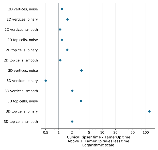
Each marker summarizes four requests: three regular sizes and one asymmetric array. Values to the right of one favor TamerOp. The logarithmic axis makes equal multiplicative differences equally spaced. The large binary top-cell advantage contributes substantially to the overall 2.18 ratio, while most 2D differences are smaller.
Actual runtimes and input sizes
The table shows the largest regular array in each family. Each time is the median across three rounds of measurements, using the middle time from each round, in seconds. Each ratio is the geometric mean of the three paired ratios, so it need not equal the quotient of the two displayed times. The complete case table is available as CSV.
| Input | Array shape | TamerOp (s) | CubicalRipser (s) | CubicalRipser / TamerOp |
|---|---|---|---|---|
| 2D vertices, noise | 6144 × 6144 | 9.90 | 11.1 | 1.11 |
| 2D top cells, noise | 6144 × 6144 | 8.94 | 9.47 | 1.09 |
| 2D vertices, binary | 6144 × 6144 | 4.53 | 7.51 | 1.61 |
| 2D top cells, binary | 6144 × 6144 | 4.34 | 6.49 | 1.49 |
| 2D vertices, smooth | 6144 × 6144 | 9.15 | 8.43 | 0.927 |
| 2D top cells, smooth | 6144 × 6144 | 9.34 | 8.45 | 0.933 |
| 3D vertices, noise | 176 × 176 × 176 | 4.57 | 15.7 | 3.46 |
| 3D top cells, noise | 176 × 176 × 176 | 6.18 | 20.5 | 3.38 |
| 3D vertices, binary | 112 × 112 × 112 | 17.9 | 5.48 | 0.313 |
| 3D top cells, binary | 112 × 112 × 112 | 0.409 | 68.4 | 165 |
| 3D vertices, smooth | 256 × 256 × 256 | 6.62 | 14.2 | 2.16 |
| 3D top cells, smooth | 256 × 256 × 256 | 6.67 | 14.2 | 2.13 |
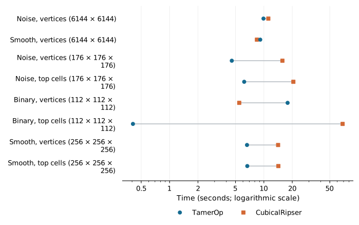
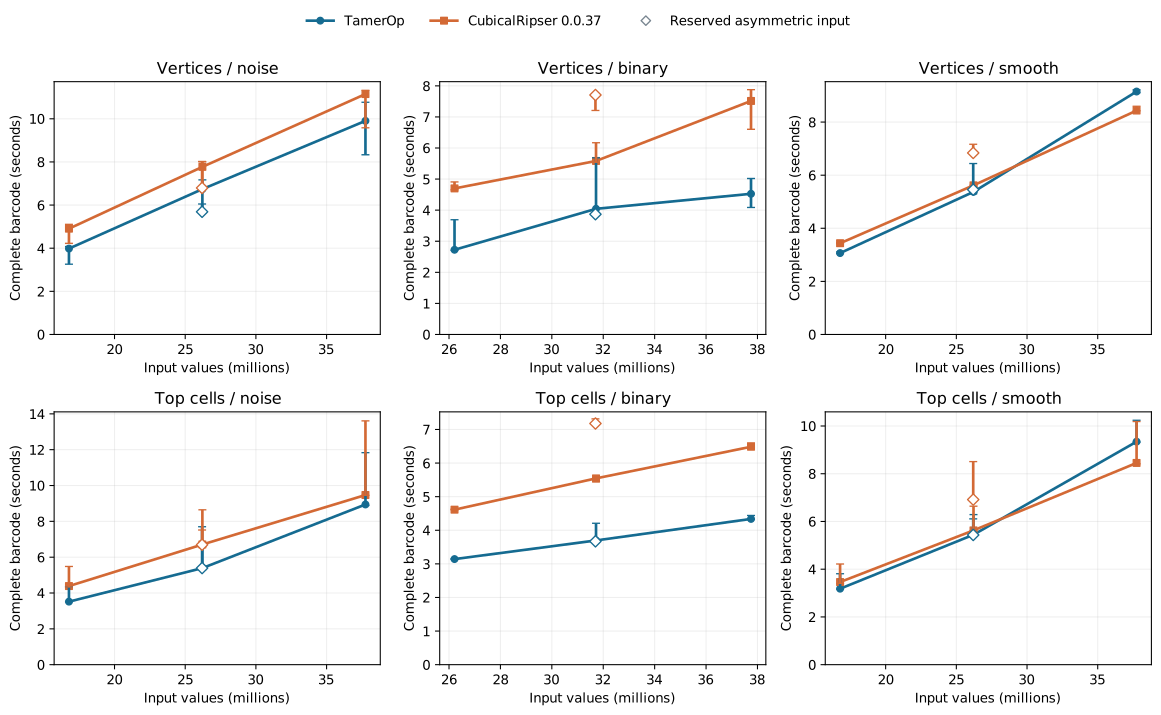
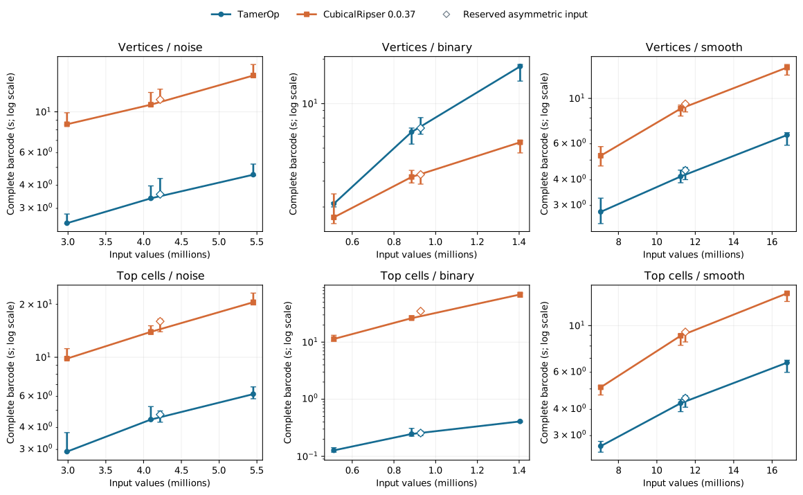
These selected rows show the waiting times behind the ratios. The 2D size curves and 3D size curves show every measured size, including the asymmetric arrays. Their vertical bars give the observed range of process medians.
What the comparison computes
A scalar image or volume determines a growing cubical complex. In the vertex convention, called V, a cell enters at the largest value of its vertices. In the top-cell convention, called T, a face enters at the smallest value of its incident pixels or voxels. These rules give different filtrations even when they start from the same array of numbers.
Both tools compute the complete ordinary barcode over F₂, the field with two elements, with nonperiodic boundaries. The answer includes every interval of positive length and every interval that persists indefinitely, retaining multiplicities. For 2D arrays it includes components and loops, the homology degrees H₀ and H₁; for 3D arrays it includes voids as well, in H₂. The array dimension describes space, while the filtration has one persistence parameter. Every measured answer agreed exactly between the tools.
The arrays contain random noise with eight possible values, binary data with two possible values, or values that increase with squared distance from the center and are rounded to integers. Each combination of dimension, input convention and structure has three regular sizes and one reserved asymmetric array, giving twelve families of four requests. The reserved arrays use separate seeds; the reserved binary and smooth cases run in superlevel order, including cells from larger values downward. These are synthetic inputs with integer grades, whose repeated values make simultaneous cell entries common.
TamerOp uses its direct cubical barcode routine. The request does not retain a finite encoded module or representative cycles. CubicalRipser 0.0.37 is called through its supported cripser.compute_ph interface. That interface also returns birth and death coordinates, so the time needed to produce those columns is included in its measurement.
How the measurements were taken
The study used the benchmark computer. The following settings identify this run:
| Component | Recorded version or setting |
|---|---|
| Date | 11 October 2026 |
| TamerOp | Frozen development source, identified by the source hashes |
| Julia | 1.12.1 |
| CubicalRipser | cripser 0.0.37, built with optimization enabled |
| Python and NumPy | Python 3.12; NumPy 2.5.3 |
| Compiler | GCC 11.4.0 |
Each program used one computation thread, with one program running at a time and other heavy computations paused. We ran three rounds, starting each input in a fresh session and taking three timings per program. A preliminary run compiles the code; each timed computation then builds the grid and calculates its barcode afresh. The programs alternate going first between inputs and rounds.
Both programs start from the same array, already loaded into memory. The timer includes building the cubical complex and returning the complete barcode. For a filtration that includes larger values first, it also includes negating the array values. Reading input files, checking answers and writing results to disk happen outside the timer.
Matching the answers
The complete barcodes agreed exactly on every measured array, including repeated intervals. Small examples were also checked with a separate barcode calculation. These exposed an incorrect component count in CubicalRipser 0.0.37 for arrays shaped 1 × 3, with values assigned to vertices, in both filtration directions. The timed arrays have at least two entries along every axis. The verification record gives the results of these checks.
Larger binary arrays and memory
Size selection used absolute runtime and resource limits. The preliminary 160³ binary vertex call took 113 s in TamerOp and 14.6 s in CubicalRipser, with matching barcodes. On the top-cell version, TamerOp took 1.31 s and CubicalRipser reached the 180 s warmup limit before a measured query completed. These single calibration samples are retained in the calibration data, separately from the repeated measurements in the main results. The final binary volume sequence uses smaller arrays.
On the 2D arrays, CubicalRipser uses up to about 7.9 GB of RAM and TamerOp about 4.2 GB. The table gives the range of maximum RAM use across the inputs in each group, measured for the whole program.
| Input group | TamerOp RAM (GB) | CubicalRipser RAM (GB) |
|---|---|---|
| 2D vertices | 2.43–4.13 | 3.53–7.92 |
| 2D top cells | 2.42–4.20 | 3.39–7.62 |
| 3D vertices | 1.29–4.20 | 0.297–2.57 |
| 3D top cells | 1.24–4.25 | 0.713–3.23 |
The data dictionary explains the memory records, including the size of the returned barcode.
Reproduce the results
The reproduction recipe gives the common procedure for verifying the downloaded evidence, recomputing summaries and figures, and preparing another measurement. The runnable CubicalRipser study includes the frozen TamerOp source, pinned competitor build and array generator. Start with these evidence files:
| File | What it contains |
|---|---|
| Data dictionary | File and field descriptions |
| Results JSON | Process medians, paired ratios, family summaries and memory measurements |
| Samples JSON | Individual measured calls and compilation counters |
| Input manifest | Array shapes, seeds, conventions and input hashes |
| Verified barcodes | Interval multiplicities for every request |
| Source hashes | The measured TamerOp source files |
| Build record | CubicalRipser source archive, build commands and binary hashes |
| SHA256 checksums | Checksums of the published evidence files |
The SHA256 of analysis.json is:
855f3917a5b6b2ea2a49c211def8009e66de928e2809f62ebb8a8c13251bf2dbThe methods explain the shared timing and comparison rules. The benchmark overview places this image and volume result beside the comparisons of persistence from point clouds and algebra on finite modules.