From source cells to representative classes
Download the executed notebook · Build and environment record
The ring in A hole appears and disappears has one loop that survives from parameter zero to five. Its interval tells us when the loop exists, but leaves room for a more geometric question: which edges form a cycle around it, and which squares fill that cycle when it dies?
We will follow the same image from its cells to a chosen cycle, a filling and a cocycle, explaining what each picture lets us conclude. A parameter atlas will then place the two homology spaces and the map between them beside those cells. Connected components provide a second example in which the source vertices themselves help us read a barcode.
The ring lesson supplies the persistence background; the installation page supplies the Julia setup. These ordinary persistence and source queries can use the filtered complex directly, without constructing an EncodingResult.
import TamerOp as OP
import CairoMakie
CairoMakie.activate!(type="png", px_per_unit=1);
See the cells that are present
The image entries give the appearance grades of square cells: the eight surrounding squares enter at zero, and the center enters at five. An edge or vertex enters as soon as a square containing it does. This is a sublevel filtration, so increasing the parameter only adds cells.
filtered_complex retains the cells, their boundaries, geometry and appearance grades. We have not asked for homology yet. Its default picture shows the first appearance parameter, which is zero here.
values = [0 0 0;
          0 5 0;
          0 0 0]
cells = OP.filtered_complex(values)
OP.visualize(cells)
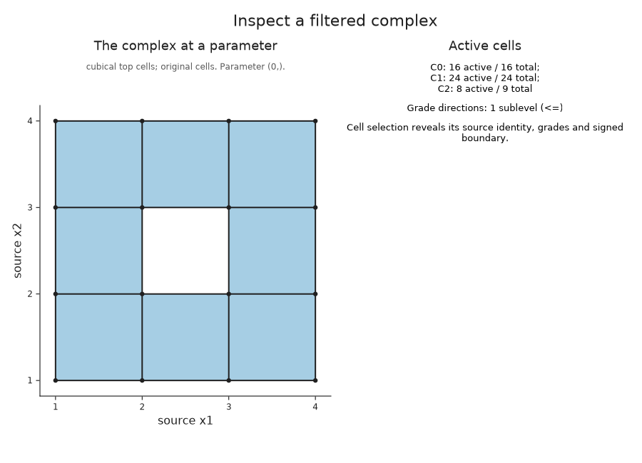
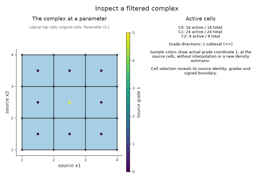
The eight squares surround a hole, and their incident edges and vertices are present too. The coordinates follow array order: the first array index gives the first geometric axis. A photograph's convention of drawing rows downward would give a different orientation of the same data.
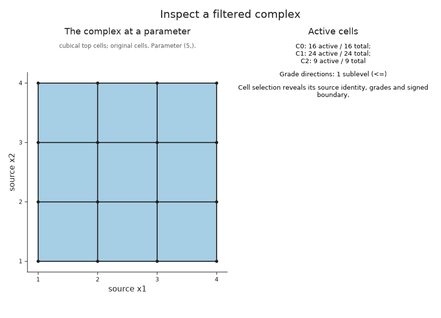
At parameter five the central square enters. Its four edges and four vertices already belong to surrounding squares, so the square count should increase by one while the other counts stay fixed.
filled = OP.Advanced.visual_spec(cells; parameter=5)
@assert filled.metadata.active_counts == [16, 24, 9]
@assert OP.Advanced.visual_spec(cells; parameter=0).metadata.active_counts == [16, 24, 8]
OP.visualize(cells; parameter=5)
Inspect a cell and its boundary
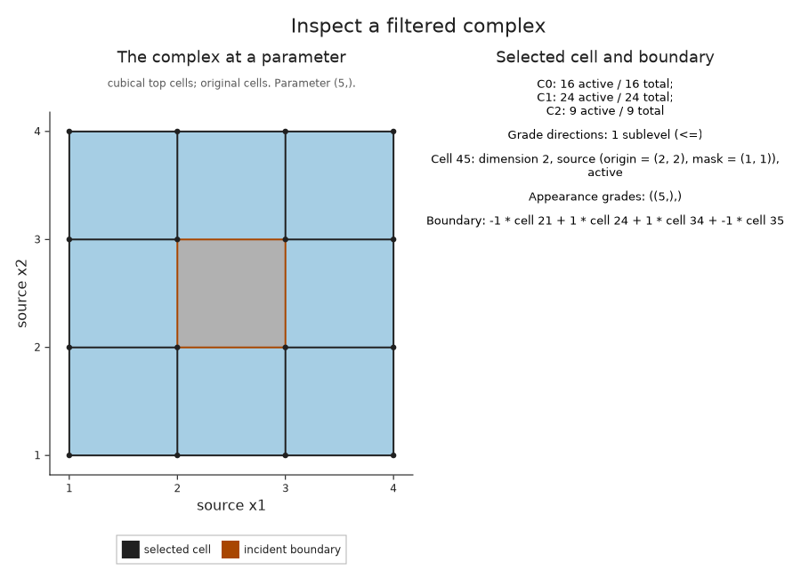
The complex viewer numbers all vertices first, then edges, then squares. In this global numbering, cell 45 is the central square. cell_source recovers its original grid location; the drawing highlights its boundary and lists the signed coefficients of its four edges.
These signs specify the integer cellular boundary before we choose a coefficient field. They tell us how the oriented edges occur in the boundary of the square. Whether that boundary represents a nonzero homology class also depends on which squares are present.
OP.Advanced.cell_source(cells, 45)
OP.visualize(cells; parameter=5, cell=45)
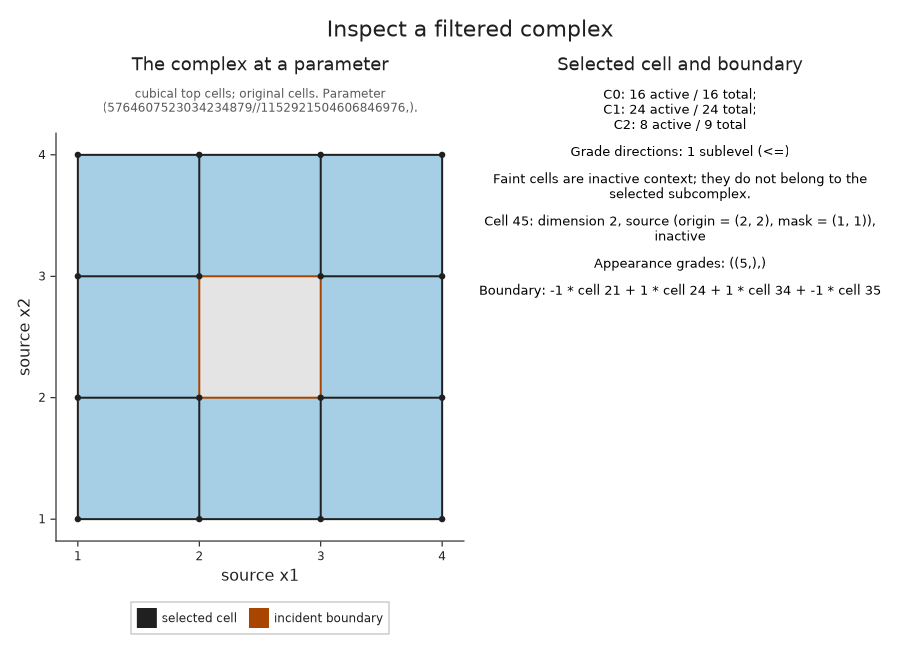
A query just below five is a useful way to separate the exact parameter from its drawing. The decimal label may round to five, but the central square must still be absent. With activity=:all, the drawing includes it faintly as context; only active cells belong to the subcomplex at the queried parameter.
just_before = 5 - big(1) // big(2)^60
before = OP.Advanced.visual_spec(cells; parameter=just_before, cell=45)
@assert !before.metadata.selected.active
OP.visualize(cells; parameter=just_before, cell=45, activity=:all)
Ask which cells represent the hole
A chain is a linear combination of oriented cells over a chosen coefficient field. Its boundary is the same linear combination of their boundaries. A cycle is a chain with boundary zero; two cycles represent the same homology class when their difference is the boundary of a chain of one higher dimension.
For the ring, we want a cycle of edges that represents its degree one interval [0,5). We retain reduction representatives with representatives=true and the correspondence to the original cells with source=true. The default field is the field with two elements, so coefficients are zero or one and signs agree. The source cell orientations are still retained, and will matter when we use another field.
The query below selects the sole finite interval and asks for its cycle at parameter two. Its source record checks that the edges are active there and that their boundary is zero.
diagram = OP.cubical_persistence(values; representatives=true, source=true)
selected = OP.Advanced.persistence_representative(diagram; dim=1, scale=2)
@assert selected.interval == (0, 5)
@assert OP.Advanced.check_source_chain(selected.source_cycle).valid
OP.visualize(selected.source_cycle)
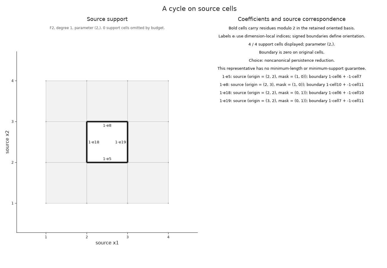
The nonzero coefficient labels tell us which source edges occur in this chosen cycle. The reduction chooses a representative; changing the order of cells with equal grades can produce another cycle in the same class.
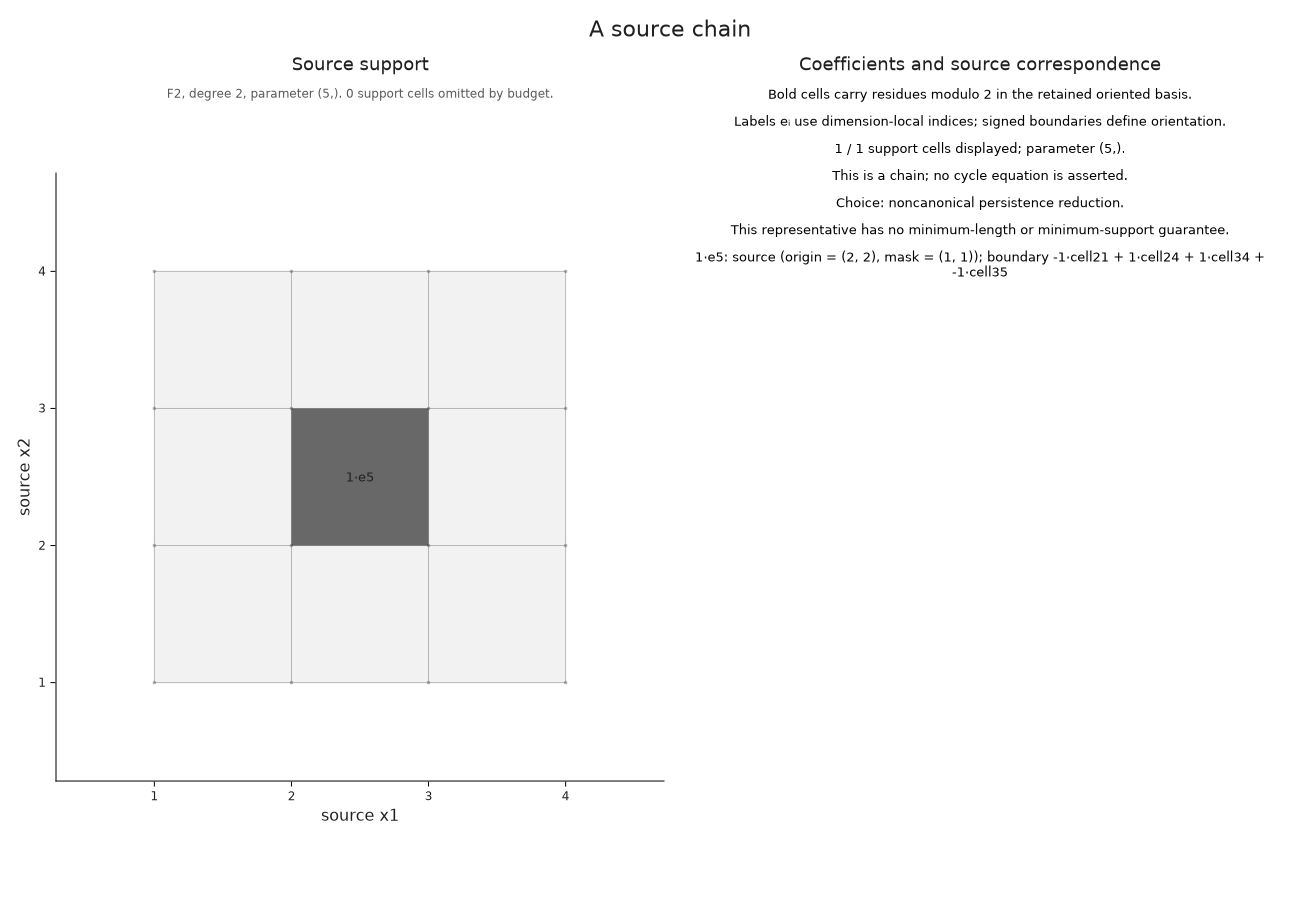
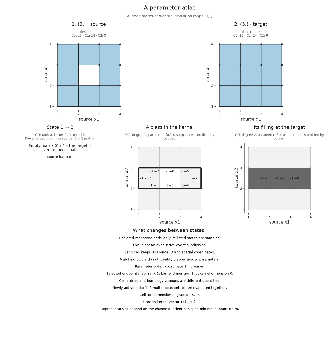
At parameter five the class dies because its cycle becomes a boundary. The returned source_bounding_chain records a chain of squares whose boundary is exactly the selected cycle. We draw that filling at death, when all of its squares are available. They need not all be present at parameter two.
filling = selected.source_bounding_chain
@assert OP.describe(filling).parameter == (5,)
OP.visualize(filling)
Measure the hole with a cocycle
A cochain assigns a field value to each cell of a fixed dimension and evaluates chains by linearity. A cocycle is a cochain that evaluates to zero on every boundary. Its value on a cycle therefore depends only on that cycle's homology class: adding a boundary does not change the answer.
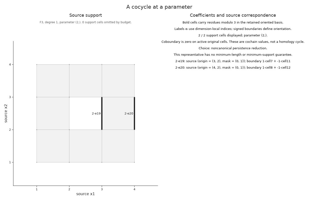
For this example we use the field with three elements. The coefficient two is minus one, so the signed orientations now affect the calculation. The returned cochain vanishes on the boundaries of all squares active at parameter two. Its finite interval excludes five, where the ring has filled.
The homology and cohomology reductions choose their representatives independently. In particular, the interval index does not identify a dual pair, and this cochain over three elements is not a numerical pairing with our earlier cycle over two elements.
cohomology = OP.cubical_persistence(values; field=OP.CoreModules.F3(), cocycles=true, source=true)
measurement = OP.Advanced.persistence_cocycle(cohomology; dim=1, scale=2)
@assert OP.Advanced.check_source_chain(measurement.source_cochain).valid
OP.visualize(measurement.source_cochain)
Keep several parameter states in view
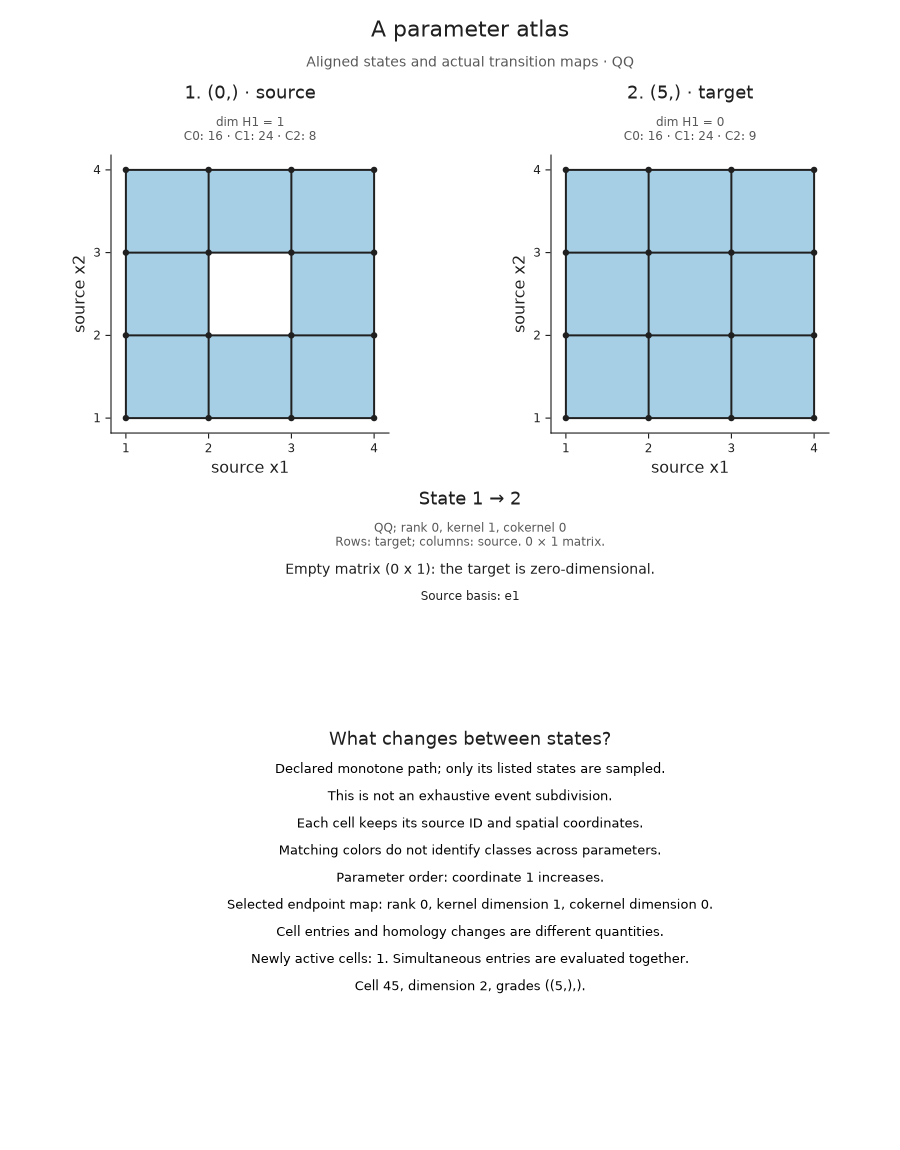
We can now compare the ring and its filled state while keeping both pictures visible. A parameter atlas in TamerOp is a declared finite collection of parameter states, together with the homology spaces and maps for the pairs that the parameter order allows us to compare. Each panel uses the same source coordinates.
We choose parameters zero and five and degree one. The atlas uses rational coefficients by default. The ring has one independent loop class over this field too, while the filled state has the zero homology space. This calculation chooses its own bases; we do not identify its representative with either of the earlier choices.
atlas = OP.parameter_atlas(cells; parameters=[0, 5], degree=1)
OP.visualize(atlas)
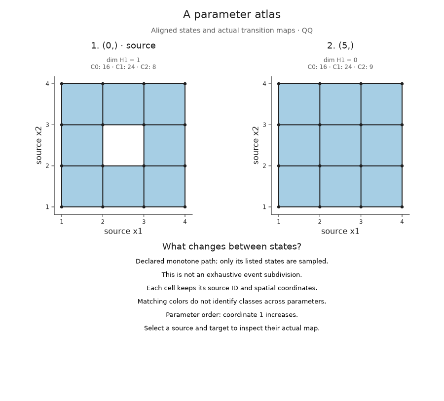
The inclusion of the ring into the filled complex induces a linear map on homology. The kernel consists of source classes that map to zero. The cokernel is the target space modulo the image, so it records target classes that cannot come from the source.
Here the source space has dimension one and the target has dimension zero. The map therefore has zero rows and one column, its kernel has dimension one, and its cokernel has dimension zero. The atlas also lists the entering cells, which answers a separate question: cell 45 is the new square that makes the loop a boundary.
State indices refer to our declared list, so state 1 means parameter zero and state 2 means parameter five. Cell 45 continues to refer to the original square.
change = OP.Advanced.atlas_transition(atlas; source=1, target=2)
@assert size(change.matrix) == (0, 1)
@assert change.kernel_dimension == 1 && change.cokernel_dimension == 0
@assert [cell.index for cell in change.entries] == [45]
OP.visualize(atlas; target=2)
To see the vanished class on the cells, request witnesses=true when constructing the atlas. A kernel witness gives a chosen cycle at the source and a chain at the target whose boundary is its included cycle. This is the same boundary equation that explained the death filling above, now obtained directly from the homology map between two parameters.
The cycle depends on the chosen homology basis and need not have minimum support. The atlas records the equation over its rational coefficient field.
explained = OP.parameter_atlas(cells; parameters=[0, 5], degree=1, witnesses=true)
OP.visualize(explained; target=2, event=:kernel)
These panels describe the chosen endpoints and their map. A loop that appears and fills strictly between two samples can leave both endpoint spaces unchanged, so this finite selection need not record every event. For several parameters, a declared grid=(xs, ys) arranges the states in coordinate order. Incomparable parameters have no prescribed transition map, even if their homology dimensions agree.
The atlas reference explains other inputs, size limits and linked selection. The retained cell example here gives the geometric meaning of its kernel cycles and fillings.
Follow whole connected components
A degree zero cycle can be a single vertex even when the component it represents contains many vertices and edges. To recover the whole component, we follow the source edges that join its vertices. component_history keeps those joins as a merge forest: leaves represent vertex births and each interior node records two components joining along an edge.
Consider two strips of squares separated by a middle strip. The outer strips appear at zero, and the strip between them appears at two. Until two there are two components; at two the middle strip connects them. Because the history retains vertex identities, selecting a bar can show the vertices belonging to that component.
islands = OP.filtered_complex([0 2 0; 0 2 0])
history = OP.component_history(islands)
@assert OP.component_count(history; scale=1) == 2
@assert OP.component_count(history; scale=2) == 1
OP.visualize(history; scale=1)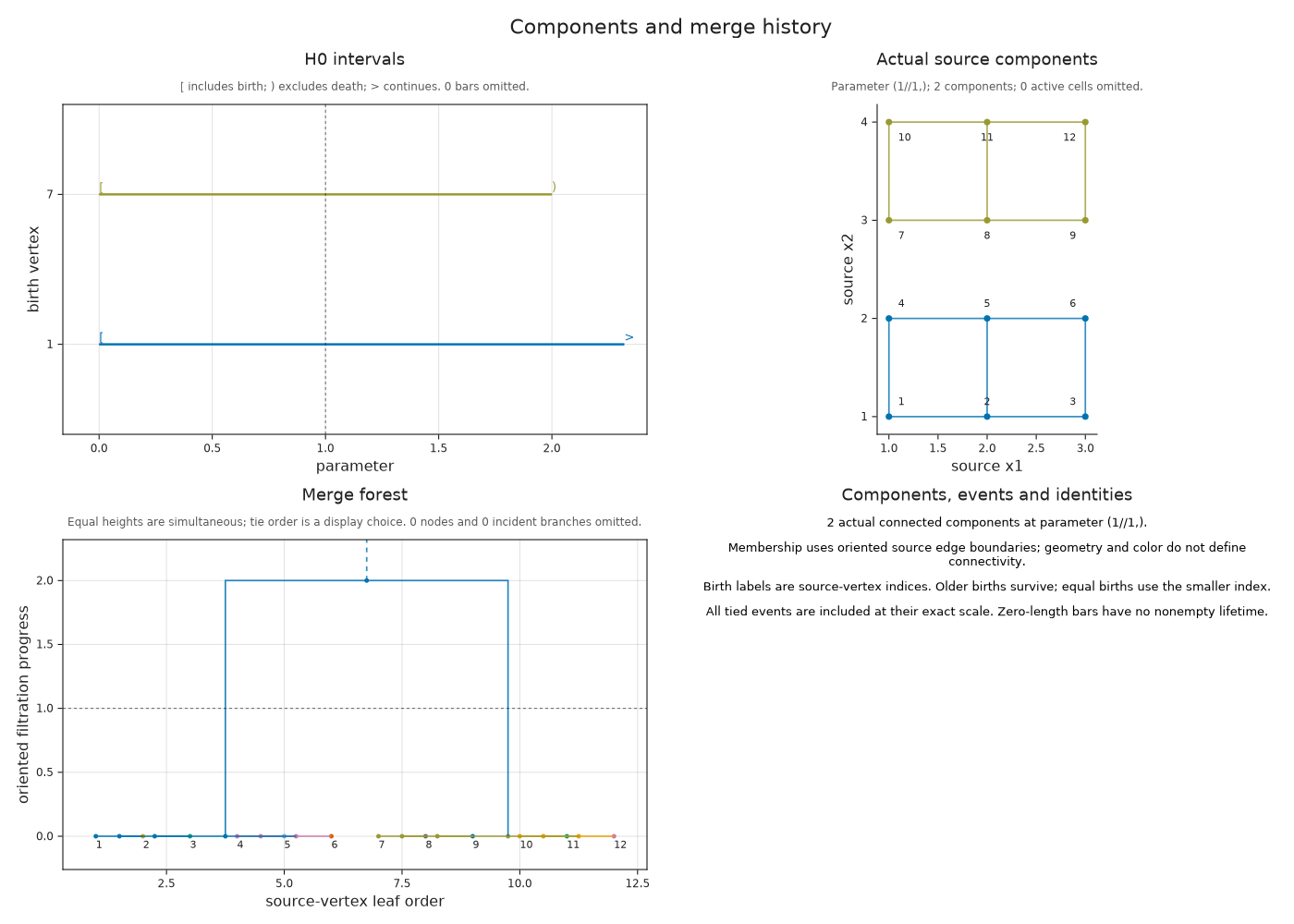
The barcode labels a component by its birth vertex. The merge forest shows which components joined, and the source panel shows the corresponding vertices and edges. Color follows the surviving birth label; source labels and selection outlines give the same correspondence without relying on color.
Select the finite bar just before its death. Its vertices still form one of the two separate strips. At death the bar ends, but those vertices remain in the complex as part of the surviving component.
finite_component = only(r.component for r in OP.Advanced.component_intervals(history) if r.death !== nothing)
just_before_merge = 2 - big(1) // big(2)^60
members_before = OP.component_members(history; scale=just_before_merge, component=finite_component)
@assert members_before.status == :alive
OP.visualize(history; scale=just_before_merge, component=finite_component)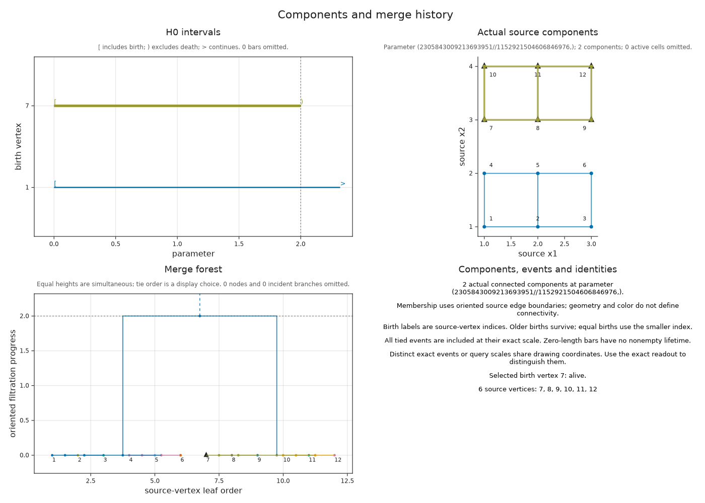
members_after = OP.component_members(history; scale=2, component=finite_component)
@assert members_after.status == :merged
@assert length(members_after.vertices) > length(members_before.vertices)
OP.visualize(history; scale=2, component=finite_component)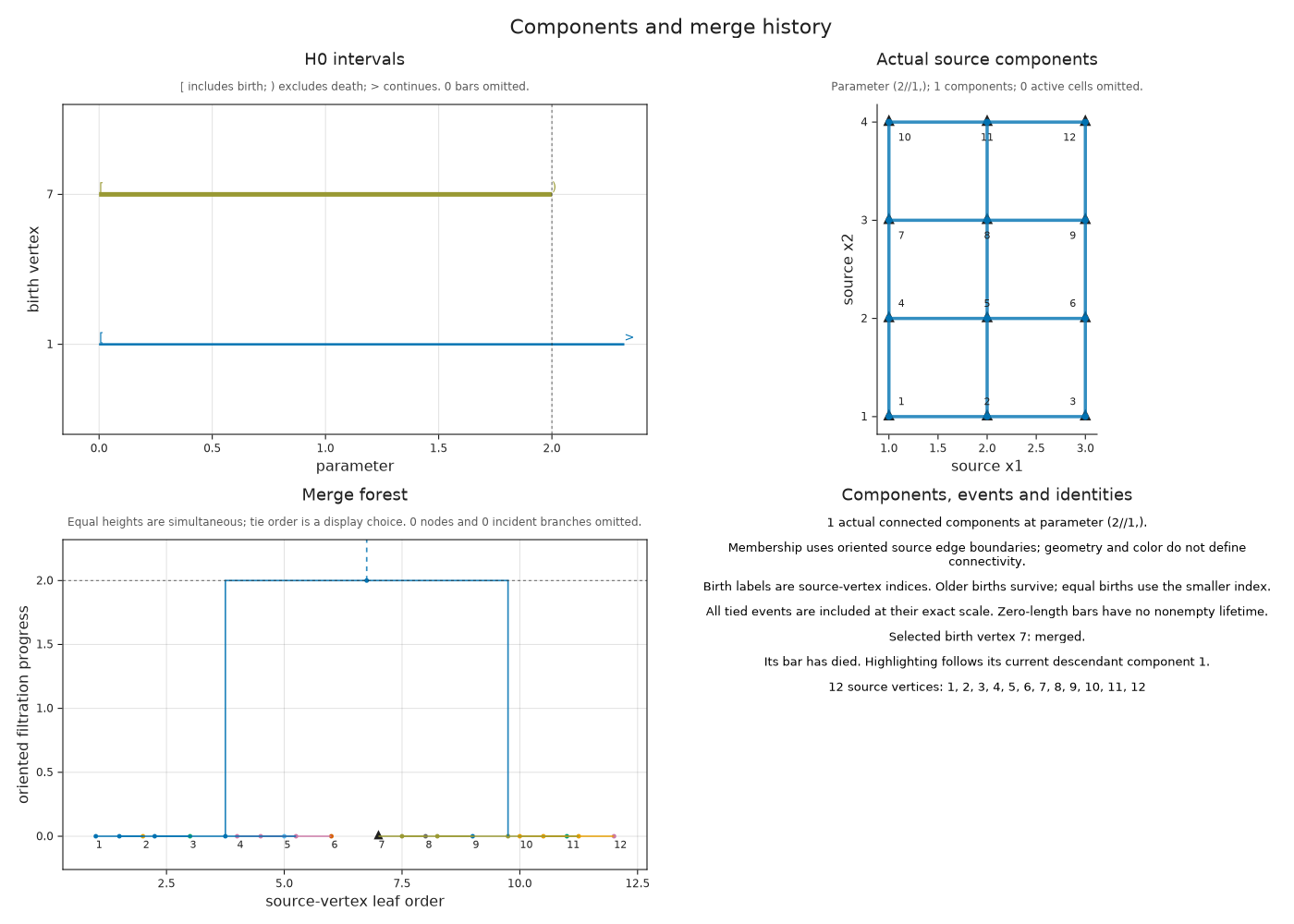
Switch between separate at parameter one and merged at parameter two in the prepared view. The same finite bar is selected in both states. Before the merge its highlighted vertices form one strip; afterward the selection follows their descendant in the joined component. Watch the source membership change while the selected interval keeps its death endpoint at two.
Both states were computed from the retained source cells. The following optional cell saves this collection as an HTML file.
Follow the selected component through its merge
Optional: Save the component views
The two prepared specifications use the same component identity and drawing coordinates. Saving them together keeps the barcode, merge forest and source membership available in a browser.
component_views = (
    separate=OP.Advanced.visual_spec(history; scale=1, component=finite_component),
    merged=OP.Advanced.visual_spec(history; scale=2, component=finite_component))
@assert OP.component_members(history; scale=1, component=finite_component).status == :alive
@assert OP.component_members(history; scale=2, component=finite_component).status == :merged
mkpath("tamerop_outputs")
OP.save_visual_session(joinpath("tamerop_outputs", "component_merge.html"), component_views;
    title="A component before and after its merge",
    caption="Separate uses parameter 1; merged uses parameter 2. The selected finite interval ends at 2, while its source vertices join the surviving component.");
At parameter two the readout says merged, and the highlighted vertices belong to the selected component's descendant. This does not extend the dead bar's lifetime. components_at(history; scale=...) returns the full partition into vertex sets, while component_count answers the counting question without listing members.
When several edges enter together, the partition after their entry is fixed but their binary merge order needs a convention. The older birth survives, with the smaller source vertex index breaking equal birth ties. The history retains births that die at the same parameter; show_ephemeral=true displays their empty bars.
Choose a slice before asking for a merge tree
For several parameters, a single increasing path makes the sequence of merges meaningful. We choose the affine line p(t) = base + t * direction, where every direction coordinate advances in its declared filtration order. The scalar t then orders the events along this line.
In the following graph, both vertices exist at (0,0), and their connecting edge appears at either (1,3) or (3,1). Such a cell is called multicritical: any one of its appearance grades suffices for entry. The diagonal (t,t) reaches an appearance grade at t=3. The line (t,2t) reaches (1,3) at t=3/2. Replacing the two appearance regions by the region above (1,1) would make the edge enter too early.
import SparseArrays
multi_graph = OP.DataTypes.MultiCriticalGradedComplex(
    [[1, 2], [3]], [SparseArrays.sparse(reshape([-1, 1], 2, 1))],
    [[(0, 0)], [(0, 0)], [(1, 3), (3, 1)]])
multi_source = OP.filtered_complex(multi_graph;
    geometry=[[(0, 0)], [(1, 0)], [(0, 0), (1, 0)]])
slanted = OP.component_history(multi_source; slice=(base=(0, 0), direction=(1, 2)))
@assert only(OP.Advanced.component_merges(slanted)).scale == 3 // 2
OP.visualize(slanted; scale=1)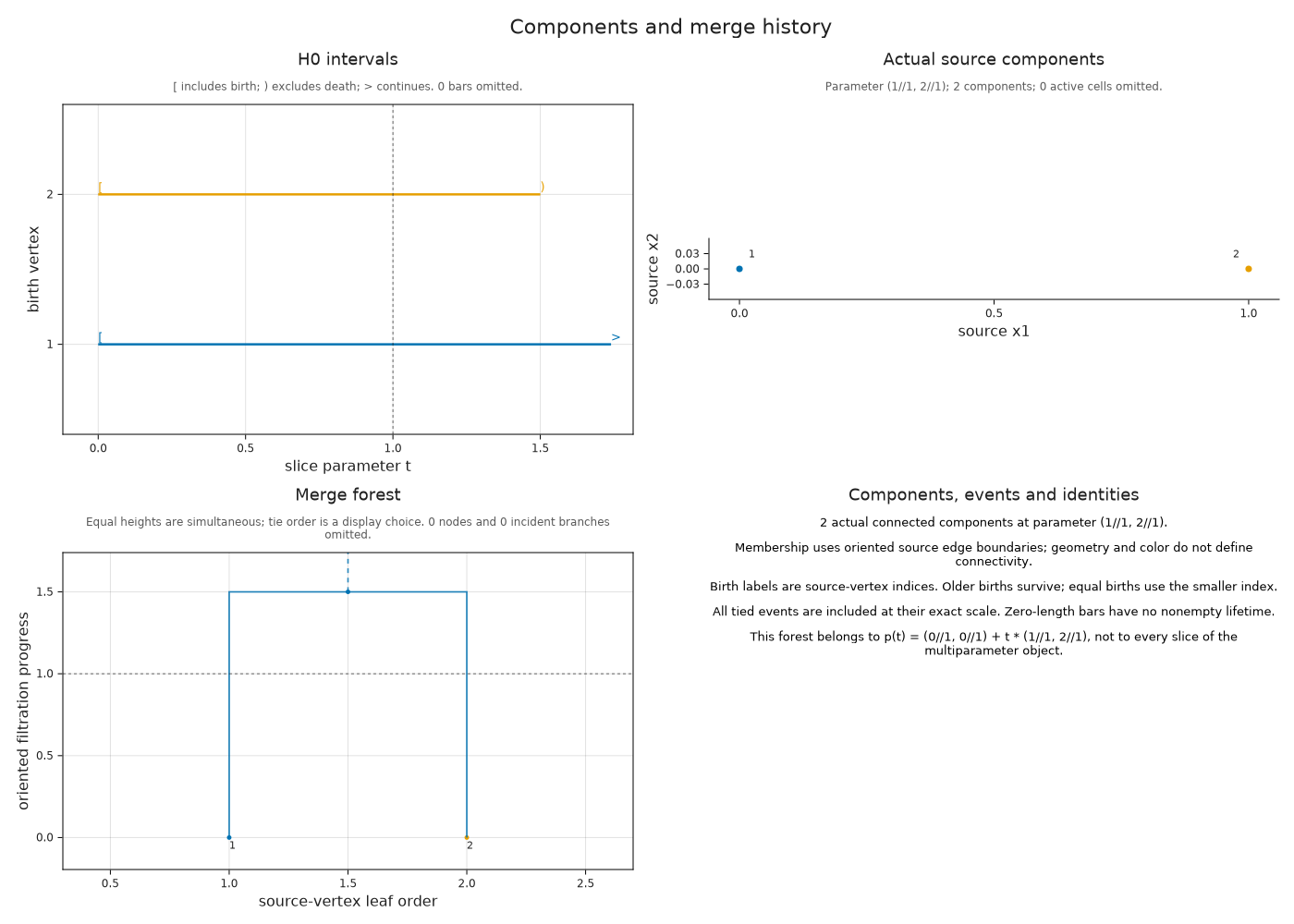
Try the diagonal direction (1,1) and predict the component count at t=2 before querying it. Both vertices are present and their connecting edge has not entered, so there are still two components. component_parameter returns the original parameter tuple for a value of t.
For a superlevel filtration, cells enter as their grade thresholds decrease. Queries still use those original thresholds, while the chart labels its increasing progress coordinate -parameter. If a persistence diagram retained its source, component_history(diagram) can recover memberships from that source and check the degree zero interval multiset. Repeated equal bars alone cannot identify the independently chosen representatives of a reduction.
Optional: Choose what a shorter representative means
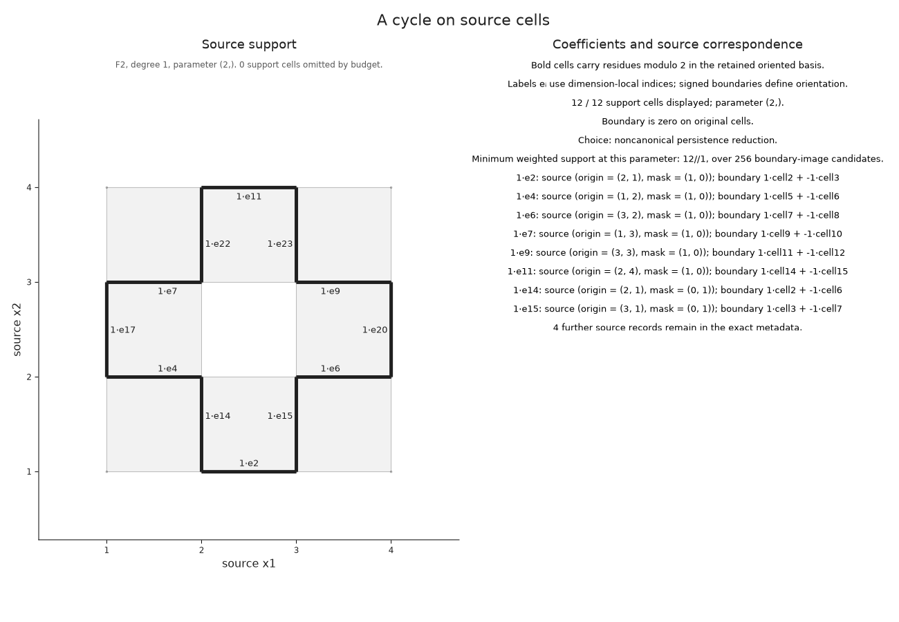
We can ask for a different representative of the ring's class while keeping the complex, field and parameter fixed. At parameter two, give the edges in our chosen cycle weight five and all other edges weight one. Minimizing the total weight of edges with nonzero coefficients then encourages another route around the hole. These weights express our preference; they are not Euclidean edge lengths.
optimize_representative enumerates the possible boundaries in the active finite complex and adds them to the original cycle. It retains the candidate of least weighted support together with a chain whose boundary is the difference. The search refuses to proceed if the number of candidates exceeds its budget. The resulting guarantee concerns this parameter and these weights; drawing a cycle never starts the search.
weights = ones(Int, OP.describe(selected.source_cycle).cell_count)
weights[collect(OP.Advanced.source_chain_data(selected.source_cycle).cell_indices)] .= 5
optimized = OP.Advanced.optimize_representative(selected.source_cycle; weights)
@assert OP.describe(optimized).metadata.nonzero_class
@assert OP.describe(optimized).metadata.objective < sum(weights[collect(OP.Advanced.source_chain_data(selected.source_cycle).cell_indices)])
OP.visualize(optimized)
Optional: Vary the input model
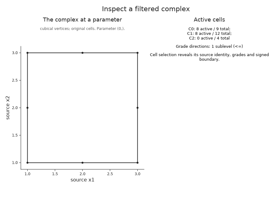
The same array can assign values to vertices rather than squares. An edge then waits for both endpoints, and a square waits for all four vertices. The high center vertex delays every edge and square containing it.
At parameter zero the resulting complex has eight vertices, eight edges and no squares. Compare it with our first ring picture. The cell models differ even though, in this example, their degree one intervals have the same endpoints.
vertex_cells = OP.filtered_complex(values; input=:vertices)
@assert OP.Advanced.visual_spec(vertex_cells).metadata.active_counts == [8, 8, 0]
OP.visualize(vertex_cells)
For the original square input, field_axis=1 adds the supplied grades at square centers. Each plotted value belongs to a cell; no interpolation or further density estimate is involved. The color scale stays fixed as the parameter changes.
OP.visualize(cells; parameter=5, field_axis=1)
Inspect a complex built from points
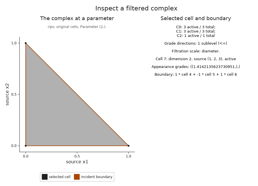
A Vietoris–Rips filtration adds a simplex when every pairwise distance between its vertices is at most the threshold. Thus the parameter measures simplex diameter. For these three points, two edges appear at one, and the third edge and filled triangle appear together at the diagonal distance $\sqrt{2}$.
The picture at threshold two contains the actual simplices from that construction, including the triangle. Selecting it reveals its three source vertices and its signed boundary.
cloud = OP.PointCloud([0.0 0.0;
                       1.0 0.0;
                       0.0 1.0])
triangle = OP.filtered_complex(cloud, OP.RipsFiltration(max_dim=2))
@assert OP.Advanced.visual_spec(triangle; parameter=1).metadata.active_counts == [3, 2, 0]
OP.visualize(triangle; parameter=2, cell=7)
Read periodic identifications and omitted dimensions
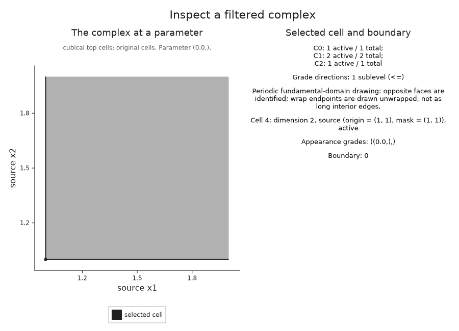
A square with opposite sides identified gives a torus. Its planar drawing is a fundamental domain: copies of the boundary stand for the same cells. Our one-square example has one vertex and two edges, since all four corners and each pair of opposite edges are identified. The two appearances of each oriented edge cancel in the square's boundary.
periodic_cell = OP.filtered_complex(zeros(1, 1); periodic=true)
periodic_view = OP.Advanced.visual_spec(periodic_cell; cell=4)
@assert periodic_view.metadata.active_counts == [1, 2, 1]
@assert isempty(periodic_view.metadata.selected.boundary)
OP.visualize(periodic_cell; cell=4)
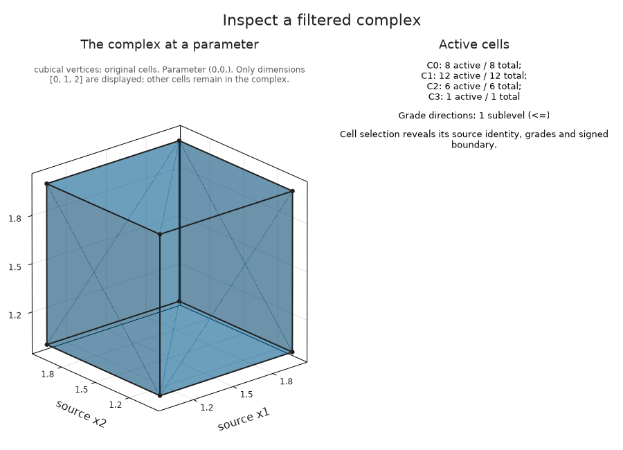
For a volume, the viewer draws cells only through dimension two, called the two-skeleton. Higher dimensional cells remain in the retained complex. This cube contains its three dimensional interior, so the visible surface is the boundary of that cell and does not represent a surviving cavity.
cube = OP.filtered_complex(zeros(2, 2, 2); input=:vertices)
@assert OP.Advanced.visual_spec(cube).metadata.active_counts == [8, 12, 6, 1]
OP.visualize(cube)
Keep a periodic class tied to its cells
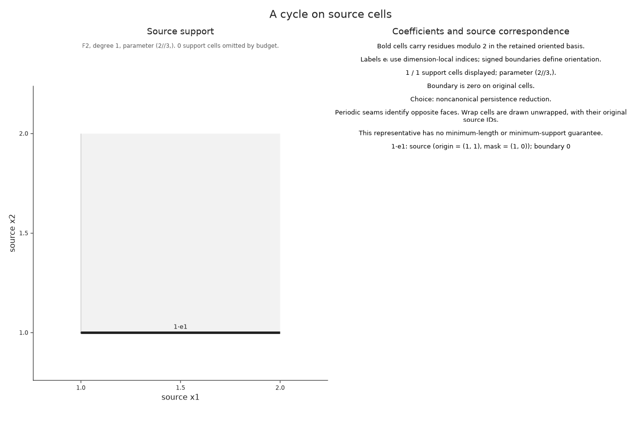
The one-square torus has two essential degree one intervals with the same endpoints. We select one original member explicitly. Its edge crosses a periodic seam and has zero boundary because its endpoints are identified. The two endpoints in the drawing still represent the same source vertex.
torus = OP.cubical_persistence(fill(2//3, 1, 1); periodic=true, representatives=true, source=true)
seam = OP.Advanced.persistence_representative(torus; dim=1, kind=:essential, index=1)
@assert OP.describe(seam.source_cycle).parameter == (2//3,)
OP.visualize(seam.source_cycle)
Optional: Explore with linked controls
In a live Julia notebook, copy this example into a code cell after loading WGLMakie:
import WGLMakie
session = OP.inspection_session(cells)
OP.visualize(session; backend=:wglmakie)
Move the parameter toward five, then use Next event to reach five exactly. This distinguishes a nearby pointer value from the event at which the center enters. The exact field accepts fractions, and the readout reports the parameter whose cells are currently shown. Select cell 45 by its index to inspect the square and its boundary. The live inspection guide explains shared controls, linked views and cleanup.
For the ordinary diagram, OP.inspection_session(diagram; dim=1) links an original interval member to its retained cycle at birth and filling at death. Enable Show retained representative after choosing a member. For the component history, OP.inspection_session(history; scale=1) links bars, source vertices and merge nodes. A selected merge identifies the joining edge and moves to its exact scale.
The atlas has a corresponding session, OP.inspection_session(explained), in which selecting a pair of states lets us inspect cell entries and retained class witnesses. Render each session with OP.visualize(...; backend=:wglmakie). When finished, call OP.Advanced.close_inspection! on it; its final static snapshot remains available.
Continue from the source question
A supplied cellular complex can use the same correspondence operations with several parameters or several appearance grades per cell. source_correspondence relates retained cell bases, and lift_source_chain checks a chain at a supplied parameter. After reducing a complex, cycles follow the retained chain map and cocycles use the retraction in the reverse direction. The implementation account explains these maps with a signed triangle calculation.
For broader module questions, the finite encoding retains spaces and maps on which we can perform algebraic operations. A source correspondence supplies additional information when we want to express a result in cells. An arbitrary encoding need not contain that correspondence. The ordinary persistence guide explains which data to retain for an interval query, and the source reference gives the precise map and optimization contracts.