Keeping a selected mathematical view
Download the executed notebook · Build and environment record
A structure map becomes easier to discuss when we can return to the parameters that selected it. Along with the figure, we would like to keep the coordinates, the matrix we read, and perhaps the module itself so that we can continue the investigation later.
We will use a module supported on a closed square, save three selections, and reopen them after closing the original inspector. Their answers are small enough to know in advance: an identity map inside the square, a one dimensional space on its boundary, and a zero space just beyond it. This lets us see what the saved file preserves. An optional variation keeps a persistence interval and its representative cycle.
The example uses Julia, TamerOp and CairoMakie; see the installation page for setup. The spaces and maps guide develops the mathematical setting, but we construct the example here. The figures below are saved output, and the links in the lesson open viewers where you can switch among our prepared selections. On a narrow screen, scroll across a figure to read its panels.
import TamerOp as OP
using CairoMakie
A = OP.Advanced
TamerOp.AdvancedStart with the object behind the picture
Let $M$ assign the rational vector space $\mathbb Q$ to every parameter in the closed square $[0,2]\times[0,2]$, and the zero vector space to every parameter outside it. The space assigned to a parameter is often called its stalk. Between comparable parameters inside the square, the structure map is the identity. Whenever either endpoint has zero space, the map is necessarily zero.
The two regions and the coefficient below form an indicator presentation. The upset contains parameters whose two coordinates are at least zero, and the downset contains those whose two coordinates are at most two. Their overlap is the square. The coefficient $1$ makes the image one dimensional there. Here A abbreviates OP.Advanced, which provides the presentation and query operations. encode constructs a module on a finite poset, a finite set equipped with a partial order, together with a classifier, the map assigning each original parameter its finite label. Retaining that classifier lets a later query recover the space at the original parameter. Indicator presentations explains why this construction gives the stated module.
options = A.EncodingOptions(; backend=:pl_backend,
    poset_kind=:signature, field=OP.CoreModules.QQField())
enc = OP.encode([A.BoxUpset([0, 0])], [A.BoxDownset([2, 2])],
    reshape(OP.QQ[1], 1, 1), options)
OP.describe(enc)
(kind = :encoding_result, poset_type = TamerOp.ZnEncoding.SignaturePoset{1, 1}, module_type = TamerOp.Modules.PModule{Rational{BigInt}, TamerOp.CoreModules.CoeffFields.QQField, Matrix{Rational{BigInt}}, TamerOp.ZnEncoding.SignaturePoset{1, 1}}, encoding_map_type = TamerOp.EncodingCore.CompiledEncoding{TamerOp.PLBackend.PLEncodingMapBoxes{2, 1, 1}, TamerOp.ZnEncoding.SignaturePoset{1, 1}, Nothing, Nothing, TamerOp.CoreModules.EncodingCache}, compiled = true, backend = :pl_backend, has_cohomology = true, has_presentation = true, module_dims = [0, 0, 1, 0], materialized = true, provenance = (category = :finite_poset_representations, base_poset = SignaturePoset(regions=4, flats=1, injectives=1), field = TamerOp.CoreModules.CoeffFields.QQField(), degree = nothing, degree_convention = :not_applicable, encoding = (map_type = TamerOp.EncodingCore.CompiledEncoding{TamerOp.PLBackend.PLEncodingMapBoxes{2, 1, 1}, TamerOp.ZnEncoding.SignaturePoset{1, 1}, Nothing, Nothing, TamerOp.CoreModules.EncodingCache}, backend = :pl_backend), window = :unrestricted, orientation = :coordinatewise, construction = (requested = :presentation_encoding, effective = :presentation_encoding, substitution = :none), discretization = (kind = :finite_encoding, filtration_values = :not_resampled), approximation = (construction = :none_requested, geometry = :backend_numerical_contract, strict_eps = nothing, effective_strict_eps = nothing, feasibility = :not_applicable), backend = (requested = :pl_backend, effective = :pl_backend), ambient_identification = :not_asserted, refinement = :single_encoding))Choose $x=(1/2,1/2)$ and $y=(3/2,3/2)$. We have $x\le y$ because each coordinate increases, and both points lie in the square. Their structure map is therefore the identity $\mathbb Q\to\mathbb Q$: the basis vector $1$ continues to the basis vector $1$, with matrix $[1]$.
We ask the classifier for the two finite labels rather than assuming their numbers. Here both parameters receive the same label. Their original coordinates still describe different points, and will remain part of the saved selection.
x = (1//2, 1//2)
y = (3//2, 3//2)
classifier = OP.encoding_map(enc)
qx = A.locate(classifier, x)
qy = A.locate(classifier, y)
dimensions = OP.dimensions(enc)
selected_map = A.structure_map(OP.encoding_module(enc); source=qx, target=qy)
@assert dimensions[qx] == dimensions[qy] == 1
@assert selected_map == reshape(OP.QQ[1], 1, 1)
(source_dimension=dimensions[qx], target_dimension=dimensions[qy], map=selected_map)
(source_dimension = 1, target_dimension = 1, map = Rational{BigInt}[1;;])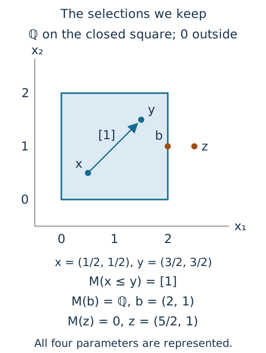
The square is the support of the module. This schematic names the selections we will save; the computed figures below also show the finite labels assigned by the encoding.
A selection joins geometry and algebra
An inspection session keeps the current query and its prepared answer together. Its snapshot is a description of the figure at that selection. In this example the three panels show the parameter regions, the module on the finite poset, and the selected matrix. The viewing box clips the drawing to a convenient size; it does not change the square or the module outside it.
We enter the pair using fractions. The selection consequently retains the exact halves, without having to recover them from a cursor's position. visual_state takes an independent copy of the prepared view and its selection, so later queries in the session leave that saved state unchanged.
For this supported inspector, the state also records how to reconstruct the query and identifies its complete mathematical source. That identity check can materialize a module whose maps were previously computed only as needed. We will use it when attaching the encoding to our saved file. An ordinary static snapshot needs less preparation when we only want a figure.
session = OP.inspection_session(enc; box=([-1, -1], [3, 3]))
A.select_inspection!(session; parameter_pair=(x, y))
inside = OP.visual_state(session)
OP.visualize(A.inspection_snapshot(session))
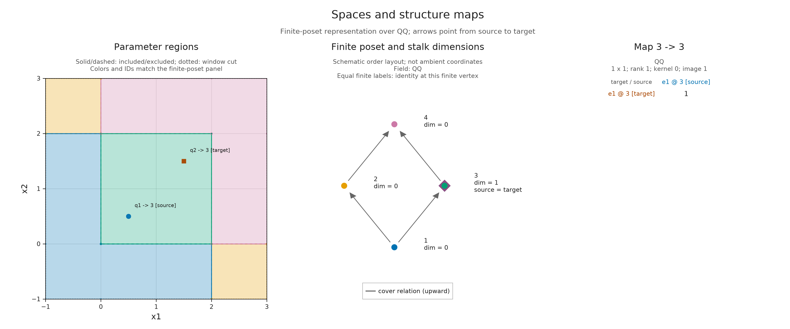
The region labels connect the first two panels: the selected parameters lie in the region whose space has dimension one. The matrix panel gives $[1]$, with its source basis along the columns and its target basis along the rows. The finite diagram's node positions are chosen for legibility; they are not another set of parameter coordinates.
Now move to $b=(2,1)$, on the square's right edge. Since the square is closed, this point still has space $\mathbb Q$. Saving it separately records the boundary convention as an exact query, even if a thick line in the picture would make nearby points difficult to distinguish.
boundary_point = (2, 1)
qboundary = A.locate(classifier, boundary_point)
@assert dimensions[qboundary] == 1
A.select_inspection!(session; point=boundary_point)
boundary = OP.visual_state(session)
OP.visualize(A.inspection_snapshot(session))
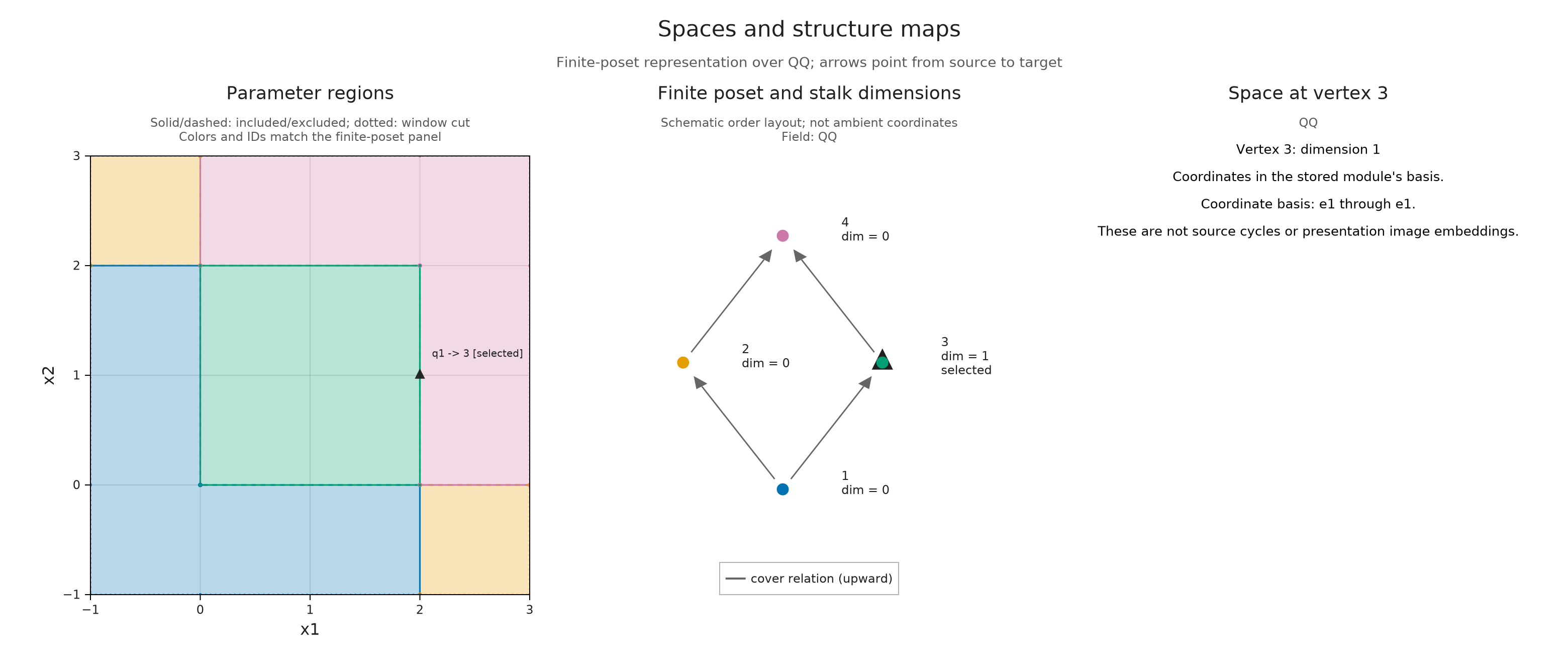
At $z=(5/2,1)$, beyond that edge, the space is zero. The classifier still returns a finite label because this encoding represents the zero space there. Its label 0 has a different meaning: a parameter with that label is outside the encoding's represented domain, so the encoding would not provide its space at all.
We keep this third selection as outside. The name refers to the square's support, the set of parameters with nonzero space. It does not mean that we have left the encoding's domain.
outside_point = (5//2, 1//1)
qoutside = A.locate(classifier, outside_point)
@assert qoutside != 0 && dimensions[qoutside] == 0
A.select_inspection!(session; point=outside_point)
outside = OP.visual_state(session)
A.inspection_selection(session)
(vertex = 4, pair = nothing, query_points = ((5//2, 1//1),), parameter_relation = :not_applicable, selector = :point, input = :provided, revision = 3, view = :module, basis = false, upset = 1, downset = 1, slice = nothing, slice_scope = :window, interval = nothing, member = 1, class_parameter = nothing, class_anchor = nothing)Keep the choices that explain your result
A saved session is a collection of named states. The names below let someone choose the interior pair, the boundary point or the point outside the support without reconstructing our sequence of queries.
We save two files to illustrate two ways of sharing this work. The JSON file includes the mathematical encoding because we pass object=enc. JSON is a structured text format; this file stores both the prepared states and the supported object needed for new queries in Julia. Before saving, TamerOp checks that the object matches each captured source and repeats the recorded queries to check their answers.
The HTML file includes the same prepared states and their drawings, but we leave out the encoding. It can be opened in a browser with Julia closed and without network access. Its selector chooses among the three answers we prepared. A fourth query would require the mathematical object and a running Julia session. These choices are independent of the filename extension: an HTML session may include its source too, as the optional interval example will show.
The files go in tamerop_outputs/live-inspection under the current working directory. Rerunning the saving cell replaces these named examples; choose a different directory when keeping another result.
Open the square viewer from the link below and choose boundary and outside to compare the exact coordinates and dimensions. The boundary still has dimension one, while the point beyond it has dimension zero. The inside selection instead shows the identity matrix between two interior parameters. The JSON download includes the encoding for the Julia calculation that follows. The website viewers show our prepared figures; to reopen a saved record in Julia, use that JSON file or the files produced by this notebook.
saved_directory = joinpath("tamerop_outputs", "live-inspection")
mkpath(saved_directory)
json_path = joinpath(saved_directory, "square.json")
html_path = joinpath(saved_directory, "square.html")
frames = (inside=inside, boundary=boundary, outside=outside)
caption = "A module supported on a closed rational square: an interior identity map, a boundary space of dimension one, and a zero space beyond the square."
OP.save_visual_session(json_path, frames; object=enc, selected=:inside, caption)
OP.save_visual_session(html_path, frames; selected=:inside, caption,
    title="Inside, on and beyond a closed square")
@assert isfile(json_path) && isfile(html_path)
(json=json_path, browser=html_path)
(json = "tamerop_outputs/live-inspection/square.json", browser = "tamerop_outputs/live-inspection/square.html")Download the square session and encoding (JSON)
We can now close the original inspector. Closing releases its callbacks, the functions that respond to control changes, and the cached results it used during exploration. Its last static snapshot remains available. To continue working from disk, we load the saved record and check the three selected coordinates before drawing the outside state.
A.close_inspection!(session)
saved = OP.load_visual_session(json_path)
@assert Set(A.visual_session_states(saved)) == Set((:inside, :boundary, :outside))
@assert A.inspection_selection(saved; state=:inside).query_points == (x, y)
@assert A.inspection_selection(saved; state=:boundary).query_points == (boundary_point,)
@assert A.inspection_selection(saved; state=:outside).query_points == (outside_point,)
OP.visualize(saved; state=:outside)
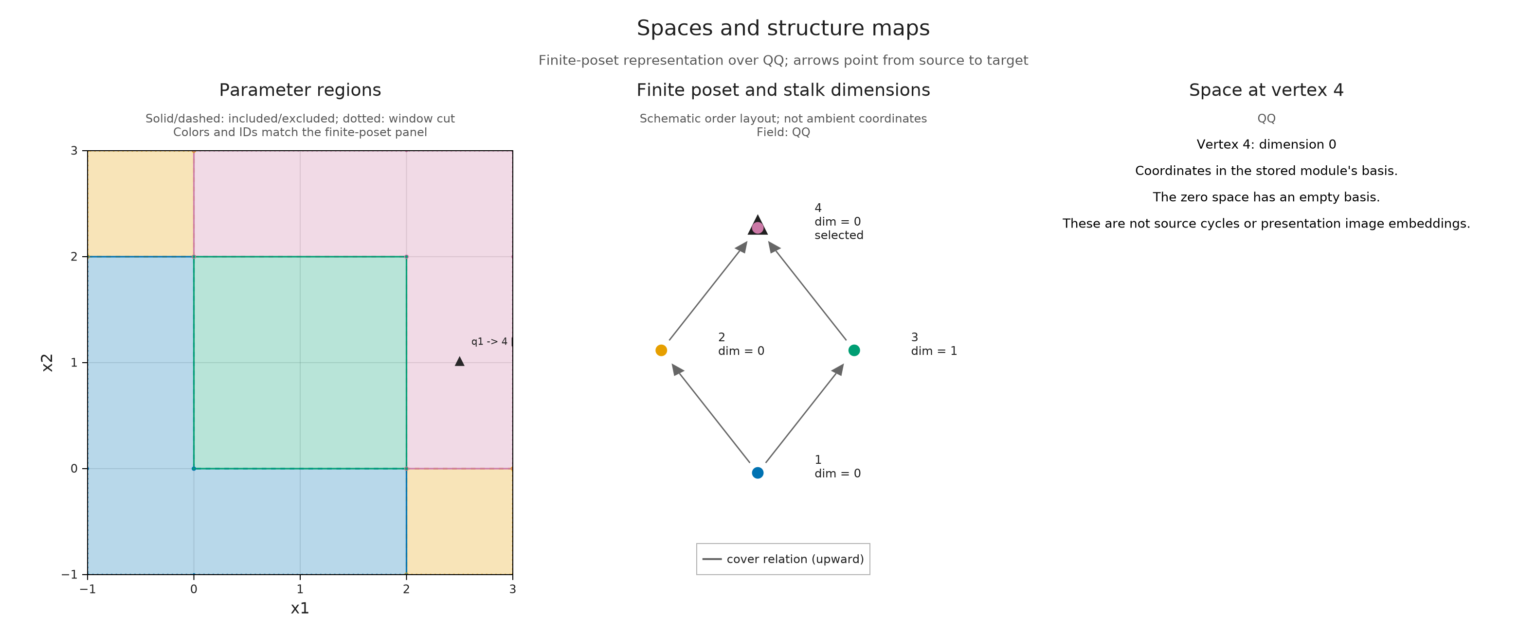
The reopened figure reports a zero space at $(5/2,1)$, as the square formula predicts. The assertions above check that the other two states have kept their exact coordinates too. Loading the record has given us the stored answers without asking the encoding a new mathematical question.
You can open the HTML file produced by this notebook and make the same selections after closing Julia. It retains the exact selected coordinates even though drawing uses numerical screen positions; each answer is already in the file.
Ask a new question in Julia
Our JSON file also contains the encoding, so inspection_session(saved) can construct a new live inspector from it. This creates new callbacks and caches; the old session remains closed. We can then select a parameter that was never one of the saved browser choices.
Before running the cell, predict the dimension at $(1/3,1/3)$. What information lets Julia answer without adding another state to the HTML file?
resumed = OP.inspection_session(saved; state=:inside)
new_point = (1//3, 1//3)
A.select_inspection!(resumed; point=new_point)
@assert A.inspection_selection(resumed).query_points == (new_point,)
@assert dimensions[A.locate(classifier, new_point)] == 1
A.inspection_selection(resumed)
(vertex = 3, pair = nothing, query_points = ((1//3, 1//3),), parameter_relation = :not_applicable, selector = :point, input = :provided, revision = 2, view = :module, basis = false, upset = 1, downset = 1, slice = nothing, slice_scope = :window, interval = nothing, member = 1, class_parameter = nothing, class_anchor = nothing)Both coordinates lie between zero and two, so the new space is $\mathbb Q$ and its dimension is one. Julia obtains the answer from the embedded encoding and its classifier. The separate HTML file continues to contain its original three states. To share this new selection, we would capture it with visual_state and save the enlarged collection.
A.close_inspection!(resumed)
nothing
Optional: preserve an ordinary interval and its representative
The same saving operations accept an ordinary persistence inspector. Consider a $3\times3$ image whose eight outer squares enter at zero and whose centre enters at five. First homology has one interval $[0,5)$: the loop exists from zero until the middle square fills it at five. The default coefficients are in $\mathbb F_2$, the field with two elements.
We retain representatives during the persistence calculation. A representative cycle is a chain with zero boundary whose homology class is the selected element. Equal intervals may be drawn as one group; selecting member=1 identifies the original interval whose cycle we want to read. A later selection cannot recover reduction data that were never retained.
image_values = zeros(Int, 3, 3)
image_values[2, 2] = 5
diagram = OP.cubical_persistence(image_values; representatives=true)
interval_session = OP.inspection_session(diagram; dim=1, window=(-1, 6))
ring_overview = OP.visual_state(interval_session)
A.select_inspection!(interval_session; interval=1, member=1, representative=true)
ring_selected = OP.visual_state(interval_session)
ring_path = joinpath(saved_directory, "ring.html")
OP.save_visual_session(ring_path, (overview=ring_overview, selected=ring_selected);
    object=diagram, selected=:selected, title="An interval and its representative",
    caption="The first homology interval [0,5) of the image ring, with its retained representative cycle.")
A.close_inspection!(interval_session)
ring_saved = OP.load_visual_session(ring_path)
@assert Set(A.visual_session_states(ring_saved)) == Set((:overview, :selected))
ring_selection = A.inspection_selection(ring_saved)
@assert ring_selection.interval == 1 && ring_selection.member == 1
@assert ring_selection.representative
OP.visualize(ring_saved)
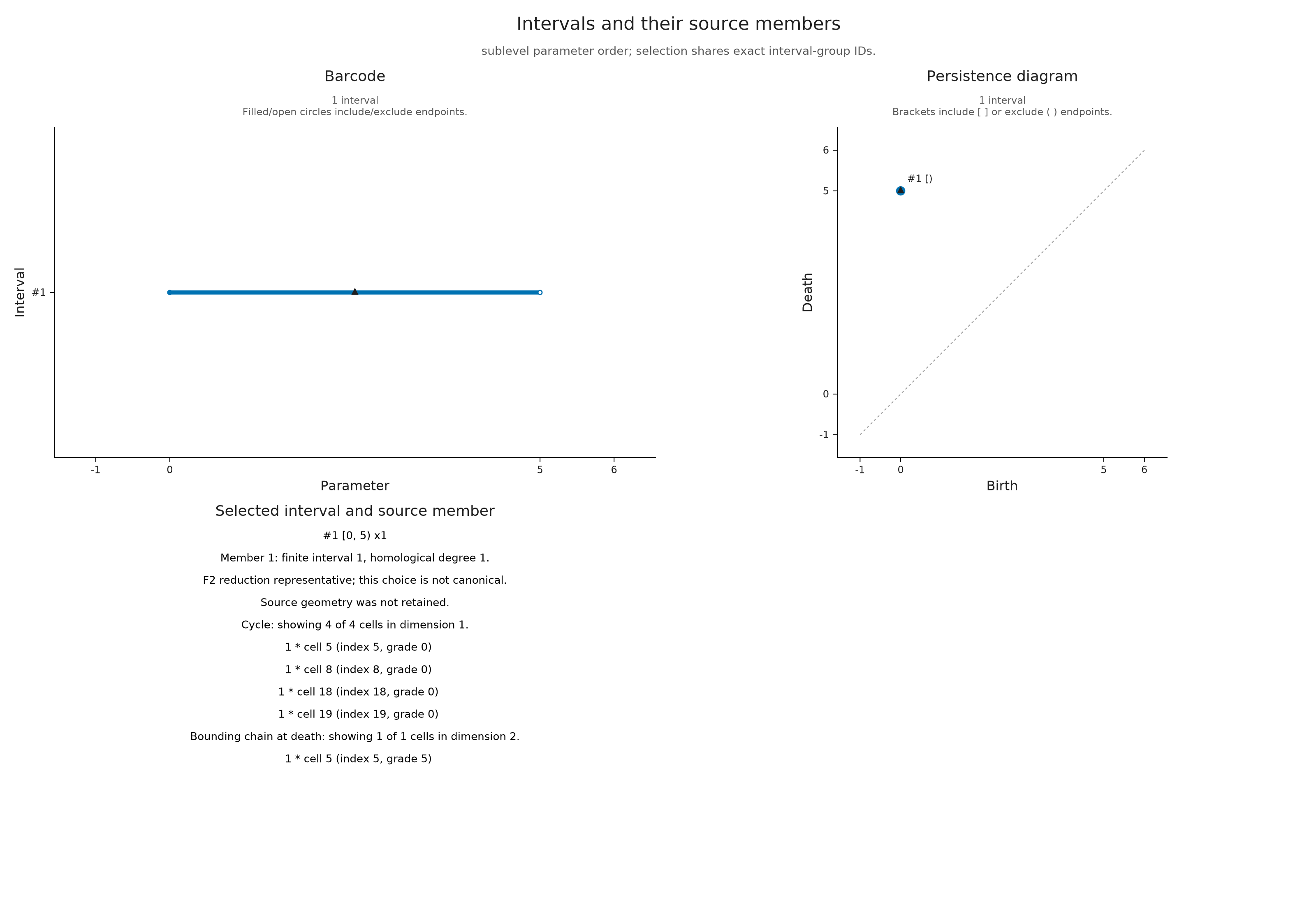
The filled left endpoint and open right endpoint show that zero belongs to the interval and five does not. The representative readout lists the edges in the cycle and the square that fills it at death, with coefficients in $\mathbb F_2$. This cycle is a choice made during reduction, so another valid calculation may choose a different representative of the same homology class.
Here we retained algebraic cell identifiers and coefficients without asking for source geometry. They let us read the chain, but do not specify where to draw its cells. The source cells lesson develops that additional geometric information.
Open the interval viewer from the link below and switch between overview and selected. The overview shows the interval before choosing a representative; the selected view adds its retained cycle and filling readout.
The HTML file saved by the notebook also embeds its diagram through object=diagram. After loading it in Julia, we can open a new interval inspector and select from the retained persistence result without recomputing persistent homology.
Explore the interval and its representative
ring_resumed = OP.inspection_session(ring_saved)
@assert A.inspection_selection(ring_resumed).interval == 1
@assert A.inspection_selection(ring_resumed).representative
A.close_inspection!(ring_resumed)
nothing
Optional: use a live browser view
The same inspector can be drawn through WGLMakie in a supported browser host while Julia remains running. Create a fresh session after loading that backend:
import WGLMakie
browser_session = OP.inspection_session(enc; box=([-1, -1], [3, 3]))
OP.visualize(browser_session; backend=:wglmakie)
Call A.close_inspection!(browser_session) when you have finished exploring. Multiple views can share that session's selection; closing one view releases its connection, while closing the session ends live selection for all of them. The display guide explains the available display modes and their requirements.
Some inspectors have continuous controls for filtration parameters or slice lines. Their readout identifies the committed choice whose answer is on screen. While Julia prepares a newer choice, the previous answer remains visible and a pending message distinguishes it from the request in progress. Rapid movements replace waiting requests, and an obsolete answer cannot overwrite a later committed selection. The source cells lesson and slice lesson show the mathematical questions behind those controls.
A cursor uses drawing coordinates, so it may be inadequate near an exact boundary. Enter the required fraction or use an event button to select a retained grade. Before calling visual_state, wait until the committed readout names the choice you want: capture records the displayed answer, not a request that is still waiting to complete. The reference gives the control and lifecycle contracts.
Decide what the recipient needs
| Intended use | What to preserve |
|---|---|
| View one selected figure | A static figure export and its interpretation |
| Switch among prepared selections without Julia | A saved HTML session with those named states |
| Read exact recorded selections and plotted values | A saved session with its selected data |
| Ask new supported questions in Julia | Captured resumable states with their matching mathematical object included or referenced |
Each state stores prepared drawing data, so more or larger views make the file larger. Capturing a resumable state also identifies its complete source, and attaching that source checks the recorded answers. When only a selected picture is needed, OP.visual_state(A.inspection_snapshot(session); selection=A.inspection_selection(session)) captures the specification and selected data without a request to reconstruct the inspector. Passing an object later does not turn that static capture into a resumable one. The session reference lists the supported reconstruction routes.
The reopening recipe gives the shorter procedure for a retained interval. Composing and sharing mathematical figures explains how to place selected views together with annotations and common scales.
The files remain in the output directory after this notebook finishes. The following optional cell lists them so we can return to the HTML viewers or load the encoding from square.json later.
Optional: List the saved files
readdir(saved_directory)
3-element Vector{String}:
 "ring.html"
 "square.html"
 "square.json"
To construct or repair the finite input itself, continue with constructing modules without a filtration. Its editor separates an editable draft from a checked mathematical object.