Working with complexes and spectral pages
Download the executed notebook · Build and environment record
A complex records vector spaces together with successive maps whose composites vanish. This condition lets us compare the vectors killed by one map with those already produced by the previous map, which is the calculation behind homology and cohomology. Resolutions and Hom computations produce such complexes, but we can begin with the matrices themselves.
We will follow a vector through a quotient, then through a map that sends its class to zero. A mapping cone will show how a related map changes degree. Finally, we will add a filtration and examine a spectral sequence, a succession of complexes that reveals how information from different filtration levels fits together.
The examples use rational coefficients, matrix kernels and quotients. The installation instructions provide the packages used below. OP.Advanced, abbreviated OA, supplies the complex constructors and inspection operations.
import TamerOp as OP
import CairoMakie
using SparseArrays
const OA = OP.Advanced
field = OP.CoreModules.QQField()
const K = OP.QQ;
Start with the differential
Consider the cochain complex in degrees 0, 1 and 2,
\[K \xrightarrow{d^0=(1,0,0)^T} K^3 \xrightarrow{d^1=(0,0,1)} K.\]
The differential $d^t$ raises the degree from $t$ to $t+1$, and $d^1d^0=0$. In degree 1, a vector $(a,b,c)$ is a cocycle when $d^1(a,b,c)=c=0$, so the cocycles form the plane spanned by the first two coordinate vectors. A coboundary is in the image of $d^0$, which is the first coordinate axis. We identify cocycles differing by such a coboundary to obtain the cohomology space
\[H^1(C)=\ker d^1/\operatorname{im}d^0\cong K.\]
The second coordinate records the class, with $(0,1,0)$ as one representative of its basis vector. For brevity we will also call cocycles and coboundaries cycles and boundaries when the degree convention is understood. Matrices use target rows and source columns; the initial view shows these differentials before requesting quotient bases.
C = OA.CochainComplex{K}(0, 2, [1,3,1],
    [sparse(reshape(K[1,0,0],3,1)), sparse(reshape(K[0,0,1],1,3))]; field)
OA.check_complex(C; throw=true)
OP.visualize(C; degree=1)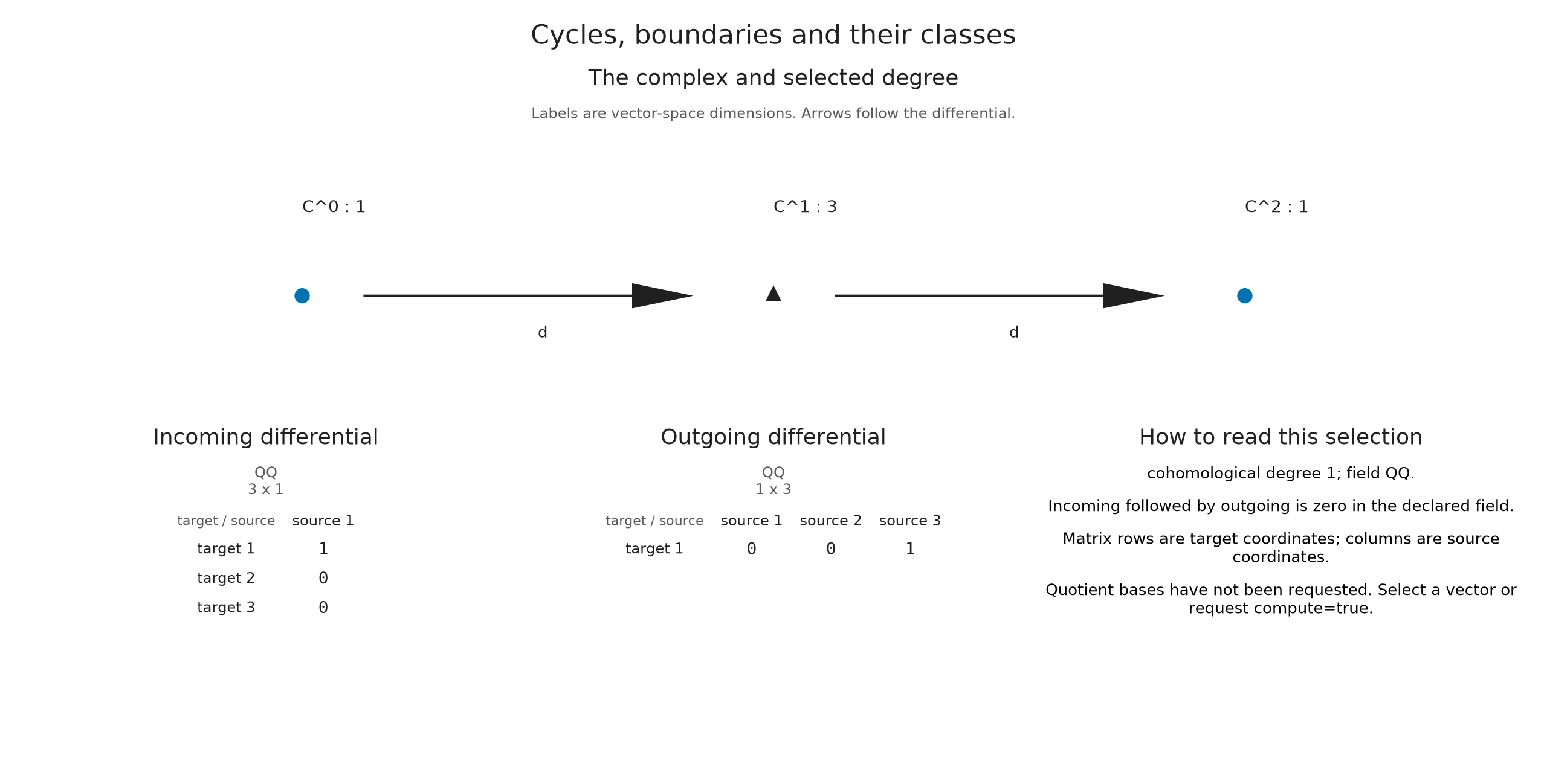
Ask what a vector represents
Take $z=(1,1,0)$. Its differential vanishes, so it is a cycle, and subtracting the boundary $(1,0,0)$ leaves $(0,1,0)$. Thus its quotient coordinate is 1 in the basis just described.
Selecting this vector requests a representative calculation. The view keeps the original vector, the quotient coordinates and the chosen representative distinct. If the chosen representative is $r$, the retained boundary adjustment $w$ explains their relation through $z=r+d^0(w)$.
z = K[1,1,0]
selection = OA.visual_spec(C; degree=1, vector=z)
s = OA.visual_metadata(selection).selection
@assert s.is_cycle && !s.is_boundary
@assert z == s.representative + OA.differential(C,0) * s.boundary_adjustment
OP.visualize(C; degree=1, vector=z)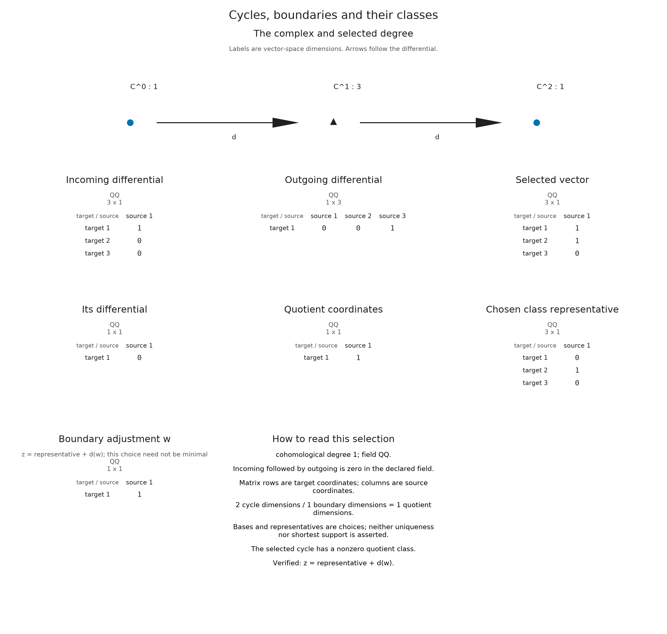
The equation is what identifies the two representatives.
We can use the same calculation to distinguish two possible failures. The vector $(1,0,0)$ is a cycle with zero class because it is a boundary. The vector $(0,0,1)$ is not a cycle at all, so it has no class in $H^1(C)$. Even when a quotient has dimension zero, its only coordinate vector, the empty vector in $K^0$, can be assigned only to cycles.
To inspect complete bases for the cycles, boundaries and quotient, request compute=true. The matrix_limit option only limits the part of a coefficient table that is drawn.
Compare a class, a boundary and a noncycle
Change the vector while keeping the degree and the two differentials fixed. For $(1,1,0)$, the differential is zero and the class is nonzero. The vector $(1,0,0)$ also has zero differential, but its quotient coordinate is zero because it is a boundary. For $(0,0,1)$, the differential is nonzero, so there is no quotient coordinate to display.
Follow a class through a map
Enlarge the incoming image to the whole cycle plane. The resulting complex $D$ has zero cohomology in degree 1. We obtain a map $f:C\to D$ by using the identity in degrees 1 and 2, and including the old boundary generator as the first of the two new generators in degree 0. These choices commute with the differentials, which is the defining condition for a cochain map.
Our selected vector $z$ is unchanged by the degree 1 map. It becomes a boundary in $D$, however, because the enlarged incoming map can now produce its second coordinate as well. The induced map on cohomology therefore sends its class to zero.
D = OA.CochainComplex{K}(0, 2, [2,3,1],
    [sparse(K[1 0; 0 1; 0 0]), sparse(reshape(K[0,0,1],1,3))]; field)
f = OA.CochainMap(C, D,
    [sparse(reshape(K[1,0],2,1)), sparse(K[1 0 0;0 1 0;0 0 1]), sparse(reshape(K[1],1,1))])
image_view = OA.visual_spec(f; degree=1, vector=z)
@assert OA.visual_metadata(image_view).map_data.target.selected.is_boundary
OP.visualize(f; degree=1, vector=z)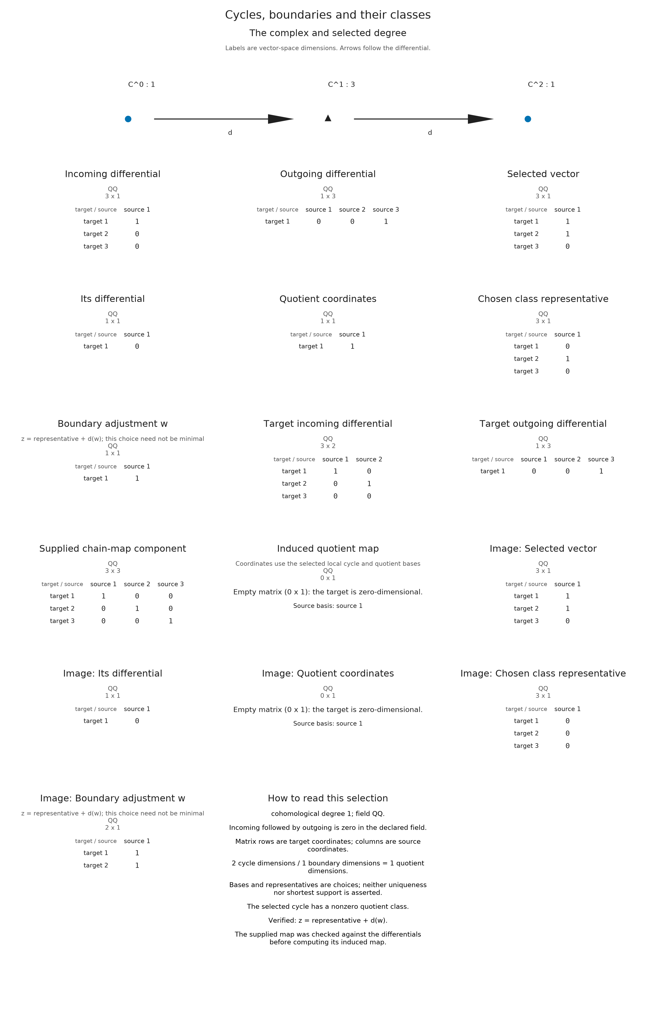
The same inspection can be performed at a vertex of a complex of persistence modules. Select vertex to obtain the complex of vector spaces there. Its displayed quotient bases belong to that stalk calculation; a separately computed cohomology module can use different coordinates. A module cochain map selects this view with kind=:chain_inspector.
If two maps $f,g$ come with a checked cochain homotopy $h$, the identity $f-g=dh+hd$ explains why they induce the same cohomology map. On a cycle $z$, the term $h(dz)$ vanishes and the difference $f(z)-g(z)=d(h(z))$ is a boundary. Supplying homotopy=H displays this witness. The chain inspection reference specifies its indexing.
For a geometric example, the source cell guide retains oriented cells and their boundaries. Its kind=:chain_inspector view uses chain degrees, so the boundary lowers degree. Vector coordinates index the active cells at the selected parameter; a retained SourceChain supplies its own parameter, field and coefficients. A position near a drawn cell is not enough to determine those data.
See a connecting map change degree
Let $E$ be a one-dimensional complex concentrated in degree 0, and let its map to the zero complex be zero. The mapping cone combines the target with a shifted copy of the source. In this case only the shifted copy remains: the cone is $E[1]$, with its line in degree $-1$.
The long exact cohomology sequence relates the source, target and cone. Its connecting map sends $H^{-1}(\operatorname{Cone})$ to $H^0(E)$, and here it is the identity. Requesting output=:full retains the maps and representatives that let us see that statement, whereas dimensions alone would only tell us both spaces are lines.
E = OA.CochainComplex{K}(0,0,[1],SparseMatrixCSC{K,Int}[]; field)
O = OA.CochainComplex{K}(0,0,[0],SparseMatrixCSC{K,Int}[]; field)
to_zero = OA.CochainMap(E,O,[spzeros(K,0,1)])
sequence = OA.long_exact_sequence(to_zero; output=:full)
connecting = OA.visual_spec(sequence; degree=-1, vector=K[1])
@assert OA.visual_metadata(connecting).selection.image_coordinates == K[1]
OP.visualize(sequence; degree=-1, vector=K[1])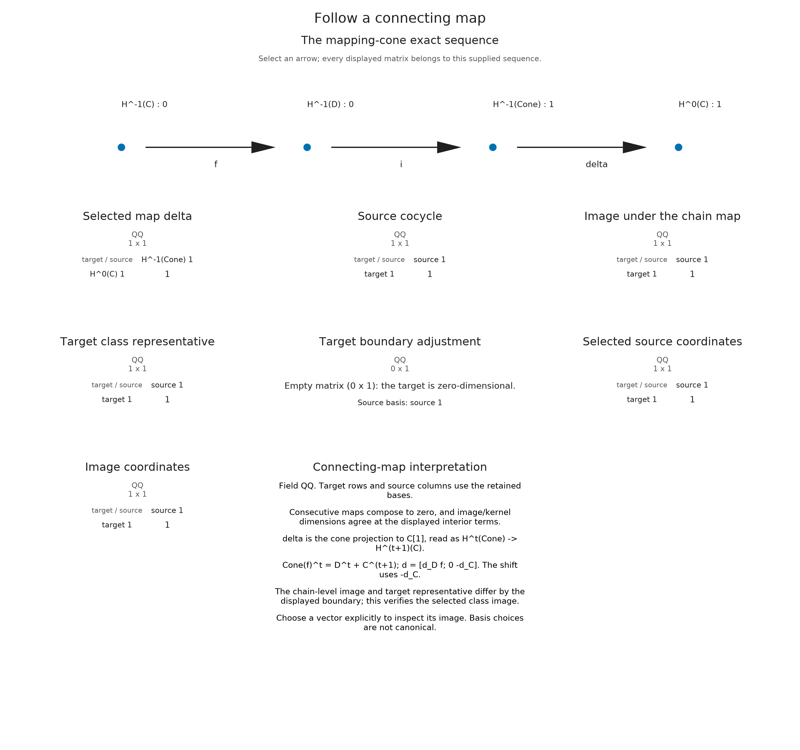
For a map $f:C\to D$, the convention is
\[\operatorname{Cone}(f)^t=D^t\oplus C^{t+1},\qquad d_{\operatorname{Cone}}=\begin{pmatrix}d_D&f\\0&-d_C\end{pmatrix}.\]
Projection onto the second summand gives a map to $C[1]$, hence the connecting map to $H^{t+1}(C)$. The sign in the shifted differential ensures that the cone differential squares to zero: its upper right block becomes $d_Df-fd_C=0$ because $f$ is a cochain map. Over a field of odd characteristic this sign cannot be discarded.
A computed result of the snake lemma offers a related view of its exact kernel and cokernel sequence. Selecting one of its five maps at a finite vertex uses the retained coordinates. The result need not retain the original commutative diagram or every lift used to derive its connecting map, so those are not reconstructed by the drawing.
Add a filtration to organize the calculation
A filtration groups a complex into nested subcomplexes. Its associated graded pieces separate the successive filtration levels, and a spectral sequence starts with these pieces before recovering interactions between levels through later differentials. Each page is a collection of spaces and maps; taking its cohomology produces the next page.
The next example shows why equal dimensions on two consecutive pages need not mean the calculation has finished. Its first differential vanishes, while its second differential removes a dimension from each of two terms.
Describe the filtered pieces
The constructor labels a piece by (p,t), where $p$ is filtration index and $t$ is total cohomological degree. A spectral chart instead uses $(p,q)$ with $q=t-p$, so total degree is $p+q$. Each of the four pieces below is $K^2$.
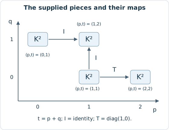
The vertical map preserves $p$ and raises $t$ by one. The horizontal maps raise both $p$ and $t$ by one. In the constructor they are supplied as d0 and d1; the figure uses $I$ for the identity and $T=\operatorname{diag}(1,0)$ for the final horizontal map. All omitted pieces and maps are zero.
These data specify a split bicomplex, meaning that the graded pieces and the two directions of differential are supplied separately. The package forms the total differential with its recorded sign convention. This constructor therefore assumes this particular two-direction description; it does not accept unspecified differential components that jump several filtration levels.
I2 = sparse(K[1 0; 0 1])
T = sparse(K[1 0; 0 0])
pieces = Dict((0,1)=>2, (1,1)=>2, (1,2)=>2, (2,2)=>2)
dc = OA.filtered_cochain_complex(K; field, pieces,
    d0=Dict((1,1)=>I2),
    d1=Dict((0,1)=>I2, (1,1)=>T))
OA.check_bicomplex(dc; throw=true)
(kind = :bicomplex, valid = true, a_range = (0, 2), b_range = (-1, 2), total_degree_range = (-1, 4), issues = String[])The first page takes cohomology along the vertical maps. The middle identity has zero kernel and cokernel, so neither of its two terms survives. We are left with $K^2$ at $(0,1)$ and $(2,0)$. A first differential moves one step to the right, and neither term has a nonzero target at that distance. Consequently the second page has the same two spaces.
ss = OA.spectral_sequence(dc; output=:full)
@assert OA.term_dims(ss; page=2) == Dict((0,1)=>2, (2,0)=>2)
OP.visualize(ss)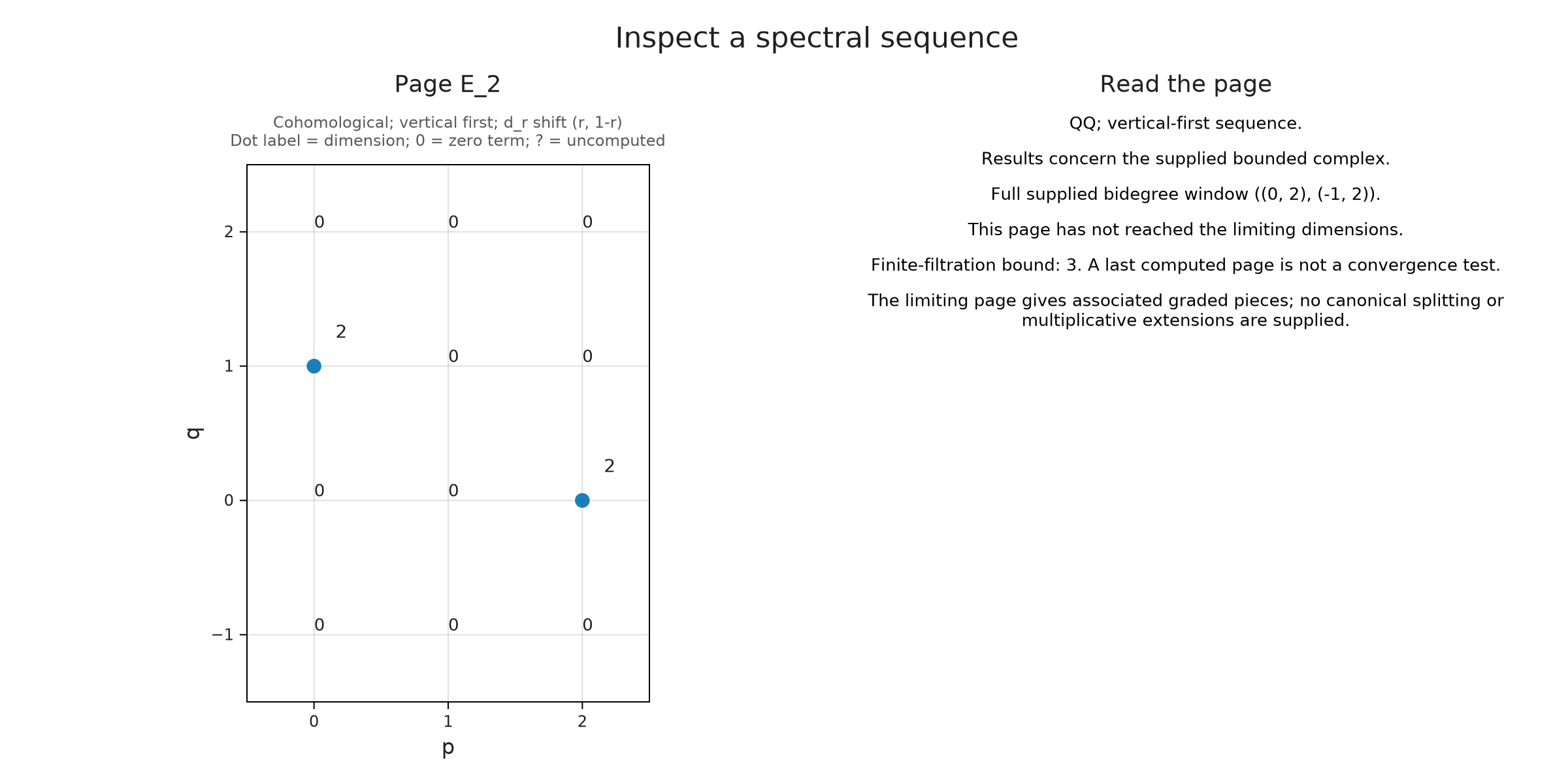
Each dot represents a vector space and its label gives the dimension. The two chart coordinates are spectral bidegrees, rather than positions in the original persistence parameter space. A computed zero term is labelled 0; a page that has not been computed is marked ?.
Inspect the map that changes the answer
A second differential moves by $(2,-1)$, so it can connect the two surviving spaces. To see its matrix, start at $(0,1)$ and follow the horizontal identity to the upper middle piece. That image can be lifted through the vertical identity from the lower middle piece. Applying its remaining horizontal map gives $T$. With the package's totalization convention this gives $d_2=T$, of rank one.
The request selects the source bidegree. The displayed matrix has target rows and source columns; the neighboring panels show its kernel and image in the selected page bases.
d2 = OA.differential(ss; page=2, p=0, q=1)
@assert Matrix(d2) == Matrix(T)
OP.visualize(ss; kind=:spectral_differential, source=(0,1))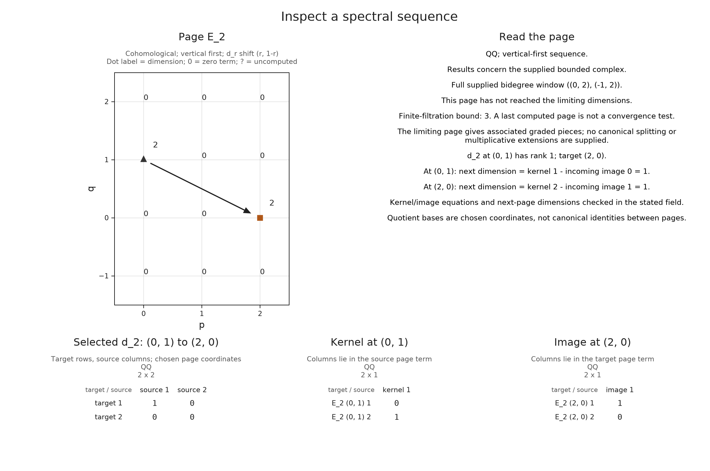
At the source, no differential arrives and the outgoing kernel is one-dimensional. At the target, the outgoing differential is zero and the incoming image is one-dimensional. Taking kernel modulo image at each location therefore leaves one dimension at each location on the third page.
The readout compares these quotient dimensions with the computed next page. Its kernel and image coordinates refer to the current page bases; they do not supply canonical identifications of individual vectors on all later pages.
@assert OA.term_dims(ss; page=3) == Dict((0,1)=>1, (2,0)=>1)
OP.visualize(ss; page=3)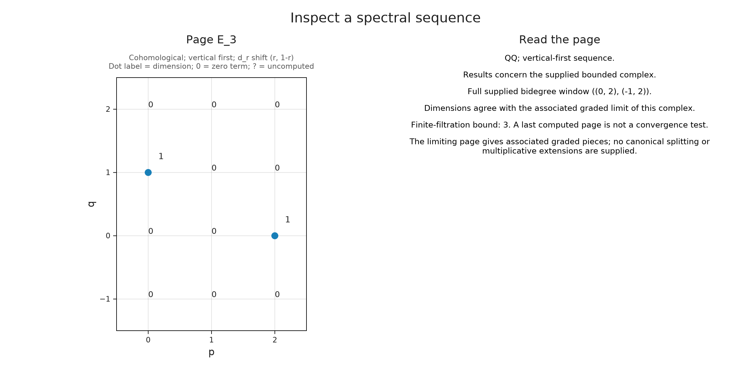
Follow the pages
Choose the first, second and third pages of this same sequence. The first two have identical dimensions, but the rank one second differential changes both surviving terms before the third page. The bidegree window stays fixed, so we can follow the change at $(0,1)$ and $(2,0)$ directly.
Read the limit without inventing a splitting
From the third page onward, a differential starting at either surviving location has no possible nonzero target in this bounded example. These terms therefore survive to the limit. TamerOp can also compute the total cohomology directly and take its associated graded pieces, giving an independent way to obtain the limiting dimensions. page=:inf requests this associated graded object.
OP.visualize(ss; page=:inf)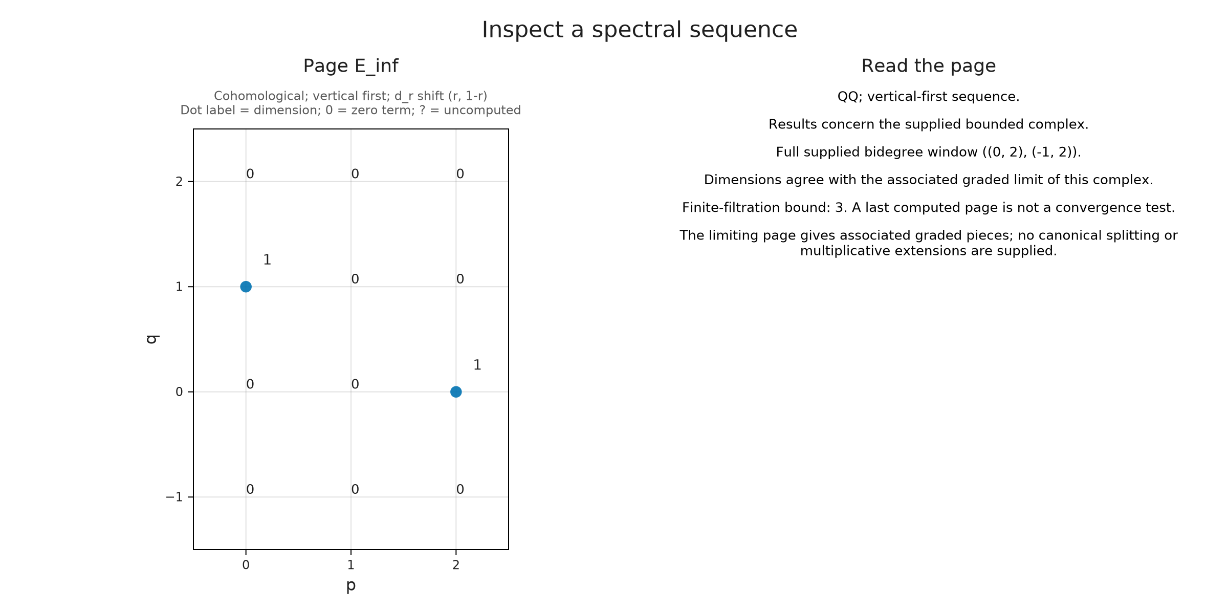
The two surviving pieces lie in total degrees $p+q=1$ and 2. More generally, several pieces can contribute to one total degree. Their dimensions add over a field, but the associated graded object does not choose a splitting of the filtration on cohomology. If multiplication is present, its extension information may also be missing from this chart.
A supplied complex may itself be a truncation of a larger intended calculation. Setting truncated=true records that limitation on the figure. By comparison, a window only selects part of the drawing: a differential can leave the visible rectangle while still contributing to the algebra. The next view deliberately displays both conventions.
OP.visualize(ss; kind=:spectral_differential, source=(0,1),
    window=((0,1),(0,1)), truncated=true)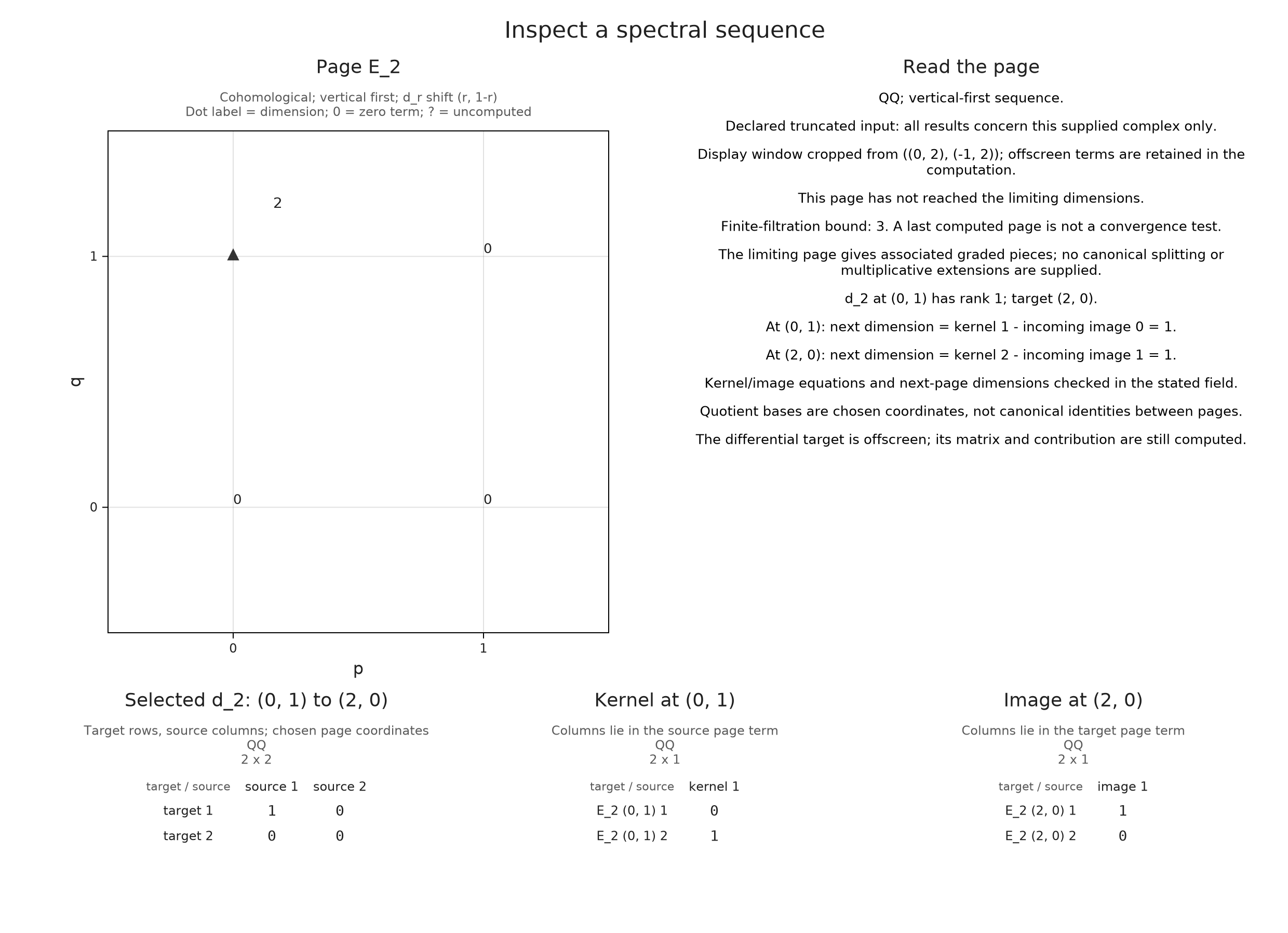
Other conventions and supplied structure
The example takes vertical cohomology first, with differentials $d_r:(p,q)\to(p+r,q-r+1)$. When horizontal cohomology is taken first, the convention is $d_r:(p,q)\to(p-r+1,q+r)$. A Tor spectral sequence reverses both bidegrees and lowers total homological degree. The viewer obtains the convention from its input, so the arrow labels stay attached to the calculation that produced them.
An independently supplied linear map between terms can be drawn as a labelled dashed line using structure_maps. Its matrix determines the arrow, and its dimensions and coefficients are checked. A label saying that it is multiplication by a class does not verify an algebra law; that requires the corresponding product data and identities. The spectral reference gives the accepted requests.
The example can be varied without changing its shape. If $T=0$, the second differential vanishes and both two-dimensional terms survive. If $T=I$, the second differential is an isomorphism and neither term survives. Construct a fresh sequence for either variation so that its computed pages refer to the new input.
The resolution guide develops another source of complexes, while the derived guide uses their cohomology classes to form Yoneda products.
Optional: prepare the vector and page comparisons
The first collection keeps only the selected vector, its differential and its quotient coordinates when they exist. The second uses the computed spectral charts on their common bidegree window. The browser changes the displayed answer; all calculations still come from C and ss above.
vector_labels = ["Nonzero class: (1,1,0)", "Boundary: (1,0,0)", "Not a cycle: (0,0,1)"]
chosen_vectors = [K[1,1,0], K[1,0,0], K[0,0,1]]
expected_cycles = [true, true, false]
expected_boundaries = [false, true, nothing]
class_views = []
for (label, vector, cycle, boundary) in zip(vector_labels, chosen_vectors, expected_cycles, expected_boundaries)
    answer = OA.visual_spec(C; degree=1, vector)
    selected = answer.metadata.selection
    @assert selected.is_cycle == cycle && selected.is_boundary === boundary
    @assert selected.differential == OA.differential(C,1) * vector
    if cycle
        @assert vector == selected.representative + OA.differential(C,0) * selected.boundary_adjustment
        drawing = OP.compose_visuals((
            vector=OP.visual_panel(answer; panel=4),
            differential=OP.visual_panel(answer; panel=5),
            coordinates=OP.visual_panel(answer; panel=6)); columns=3, title=label,
            subtitle="Degree 1 over Q; quotient coordinates identify cycles modulo boundaries.")
    else
        @assert selected.coordinates === nothing
        drawing = OP.compose_visuals((
            vector=OP.visual_panel(answer; panel=4),
            differential=OP.visual_panel(answer; panel=5)); columns=2, title=label,
            subtitle="The nonzero differential prevents this vector from defining a cohomology class.")
    end
    push!(class_views, drawing)
end
prepared_classes = NamedTuple{Tuple(Symbol.(vector_labels))}(Tuple(class_views))
complex_directory = joinpath("tamerop_outputs", "complexes")
mkpath(complex_directory)
OP.save_visual_session(joinpath(complex_directory, "vectors.html"), prepared_classes;
    selected=Symbol(first(vector_labels)), size=(1350,500),
    title="Does the vector define a nonzero cohomology class?",
    caption="In degree 1, the outgoing map reads the third coordinate and the incoming image is the first coordinate axis. All coefficients are rational.");
@assert OA.term_dims(ss; page=1) == OA.term_dims(ss; page=2) == Dict((0,1)=>2, (2,0)=>2)
@assert OA.term_dims(ss; page=3) == Dict((0,1)=>1, (2,0)=>1)
page_panels = map(1:3) do page
    chart = OP.visual_panel(ss; page, panel=:spectral_chart)
    @assert all(term -> term.status in (:zero, :nonzero), chart.metadata.terms)
    OA.VisualizationSpec(chart.kind;
        title=chart.title,
        subtitle=replace(chart.subtitle, "; ? = uncomputed" => ""),
        layers=chart.layers, panels=chart.panels, axes=chart.axes,
        legend=chart.legend, interaction=chart.interaction, metadata=chart.metadata)
end
page_views = (; var"Page 1"=page_panels[1], var"Page 2"=page_panels[2], var"Page 3"=page_panels[3])
OP.save_visual_session(joinpath(complex_directory, "pages.html"), page_views;
    selected=Symbol("Page 1"), size=(720,490),
    title="Follow the spectral pages",
    caption="Over Q, pages 1 and 2 have dimension two at both surviving positions. The rank one second differential leaves dimension one at each position on page 3.");
Explore a vector interactively
This optional exploration uses the static calculations above with a running Julia session and WGLMakie. The browser connection must stay attached to that session; the display guide distinguishes this from reopening a static export or viewing an executed notebook.
using WGLMakie
chains = OP.inspection_session(C; degree=1)
OP.visualize(chains; backend=:wglmakie)
Click a degree, enter a vector, or choose quotient coordinates. Changing degree clears the old vector because its coordinates belonged to the previous space; invalid input preserves the previous valid selection. For a connecting map, select an arrow and enter coordinates in its source. Hovering reads already prepared dimensions without requesting bases.
The same selections can be made through OA.select_inspection!. OA.inspection_snapshot(chains) returns a static view, and OA.close_inspection!(chains) releases the live controls when you are finished.
Explore pages with a live Julia session
This optional spectral exploration uses the same session interface:
using WGLMakie
session = OP.inspection_session(ss)
OP.visualize(session; backend=:wglmakie)
OA.select_inspection!(session; page=2, source=(0,1))
OA.select_inspection!(session; page=3)
OA.inspection_snapshot(session)
OA.close_inspection!(session)
The browser controls let you change page, select a term or enter its bidegree. Turning off Compute requested missing data restricts inspection to retained pages and maps; other values remain unknown. The associated graded control retains the supplied complex's scope, and invalid entries leave the last valid selection intact. Closing the session releases its live inputs and callbacks while preserving the final snapshot.