Computing generalized rank and GRIL
A finite encoding retains how vectors move through the parameter order. A region can branch, requiring a vector travelling along one branch to agree with one arriving along another. Generalized rank measures how much of these compatible choices survives the identifications imposed by the maps. We will write down this comparison as a matrix, then follow its use in signed summaries and in the generalized rank invariant landscape, abbreviated GRIL.
The distinction between the finite base and the ambient parameter space matters. generalized_rank(M; vertices=I) restricts the finite module to the selected labels. gril(M, grid; centers=..., levels=..., lengths=...) instead restricts a specified continuous extension to geometric regions in the plane. The geometry determines which finite diagram computes that restriction, so we will explain that reduction separately. Both routes reuse the encoded spaces and maps; neither reconstructs an input filtration.
The region query guide follows these questions through selected domains, matrix witnesses and linked figures.
A branching question that endpoint ranks cannot answer
Take two incomparable sources, each carrying a line, and a common target carrying a plane. If both source maps land on the same line in the plane, one class can persist consistently through both branches. If their images are different lines, no nonzero class can do so. Both modules have stalk dimensions (1,1,2) and both arrow ranks are one. Their generalized ranks on the region of three labels are one and zero.
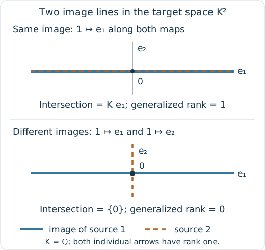
The target plane shows where vectors from the two sources arrive. The upper pair shares an entire image line; the lower pair agrees only at zero. These are vector coordinates, not positions in the parameter poset.
In the generalized rank construction of Kim and Mémoli, the limit is the space of choices of one vector at every vertex that agree under the structure maps. The colimit is the common quotient obtained by identifying each vector with its image under those maps. A compatible choice determines the same quotient class at every vertex of a connected region. The resulting linear map from limit to colimit is the comparison whose rank we want.
Write the direct sum of the selected spaces, or stalks, as
\[V=\bigoplus_{a\in I}M_a.\]
For each cover $a\prec b$, a comparable pair with no selected label between it, let $A_{ab}:M_a\to M_b$ be the structure map. The constraint matrix $C$ stacks equations $A_{ab}x_a-x_b=0$. The relation matrix $R$ has columns $\iota_a v-\iota_b A_{ab}v$, where $\iota_a$ includes one stalk into $V$. Consequently,
\[L=\ker C,\qquad Q=V/\operatorname{im}R.\]
Covers suffice because the input is a functor: all other equations and relations follow by composition. Query validation checks nonemptiness, connectivity and order convexity in the original finite poset. It does not replace the module's functoriality contract for inputs supplied by the caller.
The implementation obtains a basis matrix $B$ for $\ker C$ and a matrix $q$ with linearly independent rows whose kernel is $\operatorname{im}R$. The latter is the transpose of a nullspace basis of $R^T$. Choose any one vertex $a$ and let $E_a$ retain only its block in $V$. The returned integer is
\[\operatorname{rank}(qE_aB).\]
Connectivity makes this map independent of the anchor: across an arrow the limit equation and colimit relation identify the two choices, and an undirected path connects any two vertices. Summing over anchors would multiply the map by $|I|$; in characteristic dividing $|I|$, that would incorrectly turn a nonzero comparison into zero. TamerOp uses one anchor.
compatible vectors       one anchor stalk        common quotient class
       ker C  ----------->  M_a  ------------------>  V / im R
                project           include in V, then take the quotient
The matrices are assembled sparsely. FieldLinAlg carries out elimination over the rational numbers or a prime field, with exact arithmetic. The query rejects RealField inputs, so a numerical rank tolerance never enters this comparison. The default return value is the rank. witnesses=true retains the chosen limit basis, colimit projection and comparison matrix, accessible through limit_basis, colimit_projection and comparison_map. They express the computation in the stated coordinates; changing bases changes these matrices while preserving the rank. A zero stalk in a connected diagram forces the rank to zero, so scalar queries can stop there.
Signed reconstruction on a declared family
Suppose the caller supplies a finite family $\mathcal F$ of connected convex label sets. The supported choice compression=:total uses every space and map in each restricted diagram, rather than replacing it with selected sources or sinks. Once its ranks $r(I)$ are known, descending inclusion order gives
\[d(I)=r(I)-\sum_{J\in\mathcal F,\ I\subsetneq J}d(J).\]
This subtraction is Möbius inversion on the declared family ordered by inclusion, and guarantees $r(I)=\sum_{J\supseteq I}d(J)$ for $I\in\mathcal F$. The coefficients use integers with no fixed bit limit because repeated subtraction can exceed the range suggested by individual stalk dimensions.
For three different lines entering a plane, use the family consisting of the central vertex and the three branches, each consisting of a source and the target. The central rank is two, each branch rank is one, and the coefficients are [-1,1,1,1]. The three positive contributions add to three at the central vertex, so subtracting one recovers its dimension two. These coefficients reconstruct the specified rank queries; they make no assertion that the module splits into the listed intervals.
reconstruct_rank(summary; vertices=I) rejects undeclared queries. Other compression systems, such as source/sink compression, are also rejected: they need their own preservation hypotheses. The implemented contract is :total. In particular, the operation does not enumerate every interval; Output sizes of generalized persistence diagrams can be superpolynomial.
An optional boundary zigzag witness
A connected convex interval in a two dimensional grid admits a smaller path whose full bars recover its generalized rank. The boundary cap construction of Dey, Kim and Mémoli orders the minimal and maximal labels by their first index. Consecutive minima are joined through their coordinatewise maximum; consecutive maxima through their coordinatewise minimum. Reverse the lower path, connect its final minimum to the first maximum, and follow the upper path.
A label can appear more than once along the path, and each visit is a separate occurrence. For the middle seven labels of a grid with three labels on each axis, it visits 2,5,4,8,5,6. Both visits to 5 remain, and only adjacent path arrows and their composites impose relations. Taking the induced order on the distinct labels would construct a different diagram. Nonuniform physical axis spacing does not change this interpretation in the index lattice. The continuous worms below require a separate geometric reduction.
boundary_zigzag computes exact ranks on contiguous occurrence intervals. If $r(a,b)$ is their rank, the multiplicity of the inclusive bar $[a,b]$ is
\[m(a,b)=r(a,b)-r(a-1,b)-r(a,b+1)+r(a-1,b+1),\]
with ranks outside the path set to zero. The result checks nonnegative multiplicities, reconstruction of occurrence dimensions, and agreement of the number of bars covering the whole path with the original region rank. It stores endpoints and multiplicities without claiming an interval decomposition of the ambient module.
For $t$ occurrences this reference algorithm uses $t(t+1)/2$ rank queries, plus the original region check. Query and algebra budgets include repeated stalk occurrences. This optional witness therefore requires additional rank calculations. The cited paper uses a faster reduction on a filtration; TamerOp does not substitute that algorithm for this procedure or compute the witness when only the scalar rank is requested.
From a grid encoding to a continuous worm
The GRIL construction of Xin, Mukherjee, Samaga and Dey uses expanding closed regions around a center $p=(p_x,p_y)$. For a positive integer length $\ell$ and width $\delta\geq0$, take every closed square with sides parallel to the coordinate axes and side length $2\delta$, centered at $p+(t,-t)$ for $|t|\leq(\ell-1)\delta$. Their union is the worm. The extent along this segment is specified by its coordinate $t$, rather than Euclidean arc length. Equivalently, the worm's points satisfy
\[|x-p_x|\leq\ell\delta,\quad |y-p_y|\leq\ell\delta,\quad |x+y-p_x-p_y|\leq2\delta.\]
For $\ell=1$ this is a square. For larger $\ell$ its diagonal sides matter: a union of only $2\ell-1$ squares is a different region. TamerOp uses the continuous definition, with exact rational arithmetic for its boundaries. Floating coordinates are converted to their exact binary rational values; they are not silently rounded to a decimal grid.
The supported encoding has two strictly increasing axes and the positive product order. The module is constant on each half-open grid cell, using its lower-left label. It is zero below either first coordinate and constant along the upper tails. These extension conventions are part of the input interpretation, not an inferred boundary condition for every encoding backend. A compiled wrapper around this grid has the same meaning. General polyhedral encodings and reversed-axis grids are outside this operation's contract.
Why a finite restriction computes the continuous rank
Intersect each grid cell with the closed worm, retaining every nonempty intersection. A nonempty intersection is a rectangle, with possibly open upper sides, cut by two parallel diagonal halfplanes. When $\delta>0$ it is connected by comparability paths: within its interior, sufficiently small horizontal and vertical steps connect points, and boundary points connect to the interior by comparable steps. Degenerate nonempty intersections are points or horizontal/vertical segments and have the same property. On each intersection the module and its maps are constant identities.
All limit coordinates in one such fiber must therefore agree, and all its colimit copies are identified. Contract it to one stalk. Between different fibers, retain the original grid map whenever some point in the first is coordinatewise below some point in the second. This finite diagram gives exactly the same compatibility equations and quotient relations as the continuous restriction. Composing those relations is harmless even when a single comparable pair does not realize the composite.
The implementation decides those incidences by interval arithmetic. For a cell rectangle $[a,b]\times[c,d]$, with the actual flags for inclusion of upper endpoints, and worm band $s_-\leq x+y\leq s_+$, its $x$ projection is
\[[a,b]\cap[s_- - d,\ s_+ - c].\]
An open upper endpoint $d$ makes the second interval's lower endpoint open. The corresponding formula gives the $y$ projection. If two cells differ strictly in both grid indices, every point in the first precedes every point in the second. If an index is shared, the projected intervals determine whether an ordered pair exists. Endpoint flags distinguish an actual contact from a contact at a grid boundary excluded from that cell.
The contracted diagram enters the same constraint/relation solver as a selected finite poset query. At width zero the region consists of the center, so its rank is that stalk's dimension. A worm that enters the zero extension has rank zero.
Exact critical widths instead of a radius mesh
For fixed $p$ and $\ell$ and a positive integer rank level $k$, GRIL returns
\[\lambda_M(p,k,\ell)=\sup\{\delta\geq0: \operatorname{grank}(M|_{W(p,\delta,\ell)})\geq k\},\]
with value zero when no width is admissible. Worms are nested, and generalized rank is nonincreasing under inclusion of connected intervals.
The zero extension below the first grid coordinates bounds the answer by $\min(p_x-x_1,p_y-y_1)/\ell$ when the center is above both first coordinates. Within that bound, cell membership and incidence can change only when projection endpoints change order. Each endpoint is a minimum or maximum of affine functions of $\delta$. For the $x$ coordinate these functions are: axis coordinates; $p_x\pm\ell\delta$; $p_x\pm(\ell+2)\delta$; and $p_x+p_y-y_j\pm2\delta$. The $y$ list is symmetric.
TamerOp enumerates their positive pairwise crossings within the bound. On each intervening open interval all membership and incidence tests have fixed truth values, so the contracted diagram and its rank are constant. A query at the rational midpoint therefore determines the whole open interval. Binary search finds the last interval with rank at least $k$; its right endpoint is the exact supremum. Whether that endpoint itself attains the rank does not change the supremum. This also handles a positive rank only at width zero. Queried ranks are reused across levels at the same center and length; the output retains widths, not elimination workspaces.
For the encoding with one dimensional stalks on the quadrant $[0,\infty)^2$, centered at $(4,6)$, the widths at level one for lengths 1,2,4 are exactly 4,2,1. Level two is zero. There is no artificial upper cutoff at the grid's last label.
Costs and boundaries
For a selected region with $k$ vertices in an $n$-vertex base, the current validation and cover construction use at most $O(nk+k^3)$ order tests and $O(k^2)$ order storage. If $D$ is the sum of stalk dimensions, constraints have $D$ columns and relations have $D$ rows. Exact elimination may densify and rational coefficients may grow. Sparse assembly does not promise sparse elimination or a bound on the bytes needed to store integers of arbitrary size.
A declared family requires one rank query per member and quadratic family inclusion comparisons. GRIL validates the grid order, builds only cells meeting each worm's bounding box, and may compare quadratically many cells. Its event construction is quadratic in the number of affine endpoint expressions. Binary search uses logarithmically many interval probes per requested level, sharing already computed probes.
GeneralizedRankBudget bounds vertices, stalk dimension, potential matrix entries, order work, output/query counts, and total critical events. A bound failure raises an error; no partial landscape is presented as complete. These bounds let callers limit a selected exact query. The computation uses the explicit grid extension described above and computes widths at the supplied centers; choosing or learning those centers is a separate task.
The computations are implemented in generalized_rank.jl and gril.jl. Workflow supplies the encoding wrappers; both routes preserve the coefficient field and explicit budgets. The optional boundary witness lives in boundary_zigzag.jl.
For actual ambient interval summands, use the interval multiplicity account. Its Hom pairing with boundary data asks a different question from restriction to a selected region.