Retaining representatives and tracing them to source cells
A persistence interval tells us when a class exists. To express that class on an input image or point cloud, we need a cycle in the computed cell basis and a map from that basis to the source cells. Geometry then lets us draw the result. Interval endpoints alone do not determine any of these choices.
This account follows that map from construction to a source query. The source cells guide develops the examples and pictures, while the reference gives the calling contracts. Ordinary persistence uses these maps when source retention is requested. A supplied complex with several parameters can use the same operations at a chosen parameter without first computing a barcode.
Keep the cells and their correspondence
A FilteredComplex retains the cells, their integer boundaries, appearance grades, source identities and geometric vertices. For a cubical cell, its identity records an origin and the coordinate directions in which it extends; for a simplex, the identity is an ordered tuple of source vertices. Coefficient vectors number cells within a single dimension, while the complex viewer numbers all vertices, then all edges, and so on. The conversion uses these dimension offsets, so it depends on the cell basis even when two cells occupy the same place in a drawing.
Let $C$ be the computed chain complex and $S$ the source chain complex. A SourceCorrespondence retains a chain map $i:C\to S$. A chain map is a family of linear maps, one in each degree, that commutes with taking boundaries. When available, a second chain map $p:S\to C$ satisfies $pi=1_C$ and is called a retraction: mapping a computed chain to the source and back recovers it. Both maps are stored as sparse matrices over an exact rational or prime field. Ordinary persistence uses prime fields; direct queries on supplied complexes can also use rational coefficients.
A SourceChain is a resulting chain or cochain at one parameter, with its field, source identities and geometry. The boundary matrices determine the oriented cell basis. Projecting coordinates for a picture or printing a residue modulo a prime does not change that basis.
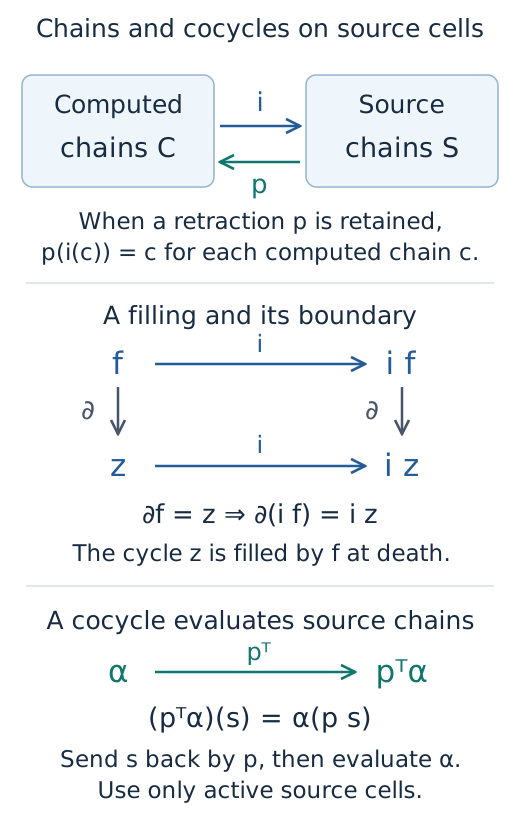
The cycle and filling follow $i$ toward the source. A cocycle follows the transpose of $p$, because it evaluates chains arriving from the source.
An ordinary diagram stores the correspondence when the caller supplies one or requests source=true. The flags representatives=true and cocycles=true retain their respective reduction data independently. A computation requesting only intervals avoids these storage costs. Retaining source cells requires an explicit complex, which can use more memory than a Rips reduction that generates simplices only as needed.
Why the maps preserve cycles
Write $\partial^C_d:C_d\to C_{d-1}$ and $\partial^S_d:S_d\to S_{d-1}$ for the boundary maps in degree $d$. The chain map condition is
\[\partial^S_d i_d=i_{d-1}\partial^C_d.\]
If $z\in C_d$ is a cycle, its source boundary is therefore $\partial^S_d(i_dz)=i_{d-1}(\partial^C_dz)=0$. If a chain $f\in C_{d+1}$ fills it, so that $\partial^C_{d+1}f=z$, the same equation gives $\partial^S_{d+1}(i_{d+1}f)=i_dz$. These equations explain why the lifted filling bounds the lifted cycle. The implementation checks them over the declared field, including signs that disappear over $\mathbb F_2$ but matter over an odd prime field.
The maps must also respect the filtration. Whenever a domain cell is present, every cell with a nonzero coefficient in its image must be present. A cell with several appearance grades is active in the union of the corresponding upper sets, using each coordinate's declared order. Checking every appearance grade of each domain cell establishes this condition throughout the filtration; checking one convenient parameter would not.
An explicit lift may be any filtered chain map. If a retraction is supplied, the equation $pi=1_C$ additionally makes $i$ injective on chains and homology: applying $p$ to an image recovers the original class. This still allows extra source classes outside the image. The automatic contraction below establishes the stronger conclusion that the complementary source cells contribute no homology.
Recover a retraction after removing cells
For a computed subcomplex, matching exact source identities first gives an inclusion in the original selected model. Its signed boundaries must agree with the source boundaries. Sampling and sparsification already determine this model; recovering cells removed by a collapse does not recover discarded points or edges omitted before the collapse.
To construct the retraction, the algorithm cancels complementary cells in pairs with equal sets of appearance grades. Suppose an extra cell $b$ has an extra face $a$ with invertible boundary coefficient $u$. In a boundary matrix $D$, the column $D[:,b]$ describes the boundary of $b$, and the row $D[a,:]$ describes the coefficients of $a$ in all boundaries. Eliminating that pair updates the remaining entries by
\[D'=D-D[:,b]u^{-1}D[a,:],\]
followed by discarding the canceled row and column. This matrix operation is a Schur complement. The accumulated projection onto the remaining chains is updated by the same cancellation. Because the target cells form a subcomplex, the projection fixes them pointwise. Equal appearance grade sets keep the cancellation valid at every parameter, including when some grades are incomparable. If complementary cells remain with no admissible cancellation, construction requires explicit maps instead of assuming that equal barcodes supply a correspondence.
For a small signed example, start with the filled triangle $[1,2,3]$ and retain the path with edges $[1,2]$ and $[2,3]$. Removing the face and edge $[1,3]$ gives a retraction with
\[p[1,3]=[1,2]+[2,3],\qquad p[1,2,3]=0.\]
The triangle boundary is $[2,3]-[1,3]+[1,2]$, so its image under $p$ is zero, as required by the chain map equation. A cochain taking values $(1,0)$ on the path edges evaluates an original edge by first applying $p$. On the ordered source edges $([1,2],[1,3],[2,3])$, its values are consequently $(1,1,0)$. Applying it to the triangle boundary gives $0-1+1=0$ over every supported prime field.
The ingestion collapse detector uses filtration domination of flag graphs; see Alonso, Kerber and Pritam. The matrix contraction described here is a further package computation on the explicit complexes. The graph detector itself does not supply these lifting matrices.
Check a cycle, its filling and a cocycle
An ordinary cycle query uses the requested parameter, or birth when none is supplied. A finite death filling uses the death parameter. Its equation $\partial f=z$ links the two records even when the filling's cells were absent at the earlier parameter. Changing the reduction order can change the chosen cycles without changing the barcode.
A cochain evaluates chains. Given a computed cocycle $\alpha$, its source value on a chain $s$ is $\alpha(ps)$, so its coordinate vector is $p^*\alpha=p^{\mathsf T}\alpha$. This is the contravariant direction: the cochain moves opposite to the map $p$ on chains. The lift $i$ has the wrong direction for this operation. The implementation restricts the returned cochain to active source cells and checks that it evaluates to zero on every active boundary. Homology and cohomology reductions choose their bases independently, so equal interval member indices do not establish dual bases.
These checks use boundaries and grades before converting coordinates for drawing. A periodic edge can have zero boundary even though its two endpoints look distinct in a planar fundamental domain: those endpoints are identified. The drawing preserves that seam. Higher dimensional chains remain available as algebraic records, while source overlays draw degrees zero through two.
Recover connected components from their merge history
For degree zero, the source vertex and edge incidences determine component membership. component_history orders edges by their exact entry parameters and maintains a partition of the vertices, joining the two parts whenever an edge connects them. This partition algorithm is commonly called union-find. The older component birth keeps its label, with source vertex order breaking equal birth ties.
A separate binary forest records each joining edge and its parameter, with the two former components as children of a merge node. An edge whose endpoints are already joined creates no merge, nor does a periodic loop with zero boundary. Several nodes may have the same parameter when edges enter together; their reproducible binary order does not introduce distinct event times.
A query cuts this forest after all events at its parameter. Counting the remaining components does not require listing their vertices. A membership query follows each selected branch to its vertex leaves. The forest therefore uses space linear in the number of source cells, while storing a complete member list at every merge could use quadratic space. Following a birth vertex after its bar has died returns the current descendant component and records that the original bar is merged.
For several parameters, first choose an affine slice $b+tv$, where $b$ is the base point and $v$ its direction. Let $o_j$ be $1$ for a sublevel coordinate and $-1$ for a superlevel coordinate. We require $o_jv_j>0$ in every coordinate. A cell with appearance grade set $G$ enters at
\[t_{\mathrm{entry}}=\min_{g\in G}\max_j \frac{o_j(g_j-b_j)}{o_jv_j}.\]
For one grade, the maximum is the first time every coordinate has reached that grade. Taking the minimum over grades implements the rule that any one appearance suffices. The resulting merge forest belongs to this slice. When a source correspondence is supplied, the operation additionally compares source and computed degree zero interval multisets before returning source memberships; equal intervals alone cannot identify individual reduction choices.
Minimize support within one homology class
At a fixed parameter, all cycles homologous to $z$ have the form $z+\partial_{d+1}f$. Choose independent columns of the active boundary matrix and put them in $B$. If $B$ has rank $r$ over $\mathbb F_p$, its image contains exactly $p^r$ vectors. The optimizer checks that $z$ represents a nonzero class, checks this number against the candidate budget, and enumerates the image.
For nonnegative cell weights $w_j$, the objective is
\[\min_{x\in z+\operatorname{im}B}\sum_{j:x_j\ne0}w_j.\]
Only nonzero support contributes: the weight does not measure coefficient magnitude. Integer and rational weights remain exact, while floating weights are compared as their represented binary rational values. The result retains the original chain and a chain $f$ satisfying $x-z=\partial f$. This certifies that the nonzero homology class is unchanged.
Changing the parameter can change the available boundaries, so the minimum belongs to the declared parameter and finite source model. The enumeration has exponential cost and a hard candidate budget. Ordinary drawing and selection do not invoke it.
Explain a transition between sampled parameters
A parameter atlas asks which classes survive from a declared parameter $p$ to a comparable parameter $q$. On a retained filtered complex, each cell has the same identity at both parameters. Appearance grades and coordinate orders determine which cells are active before any drawing coordinates are computed.
In degree $d$, restricting the source boundary matrices to active cells gives
\[C_{d+1}(p) \xrightarrow{D_{d+1}(p)} C_d(p) \xrightarrow{D_d(p)} C_{d-1}(p).\]
Homology is $\ker D_d(p)/\operatorname{im}D_{d+1}(p)$. The computation chooses cycle columns $Z_p$ representing a basis of this quotient. A sparse matrix $I_{pq}$ sends each active source cell to that same cell at the target. Expressing $I_{pq}Z_p$ in the target homology basis gives the induced map $A_{pq}$. These endpoint bases remain fixed for every pair, so map compositions can be compared by matrix multiplication.
For the ring followed by its filled center, degree one dimensions are one and zero. Thus $A_{pq}$ has zero rows and one column. A vector $v$ in its kernel lifts to the source cycle $z=Z_pv$. Because this class maps to zero, a target chain $f$ satisfies
\[D_2(q)f=I_{pq}z.\]
With witnesses requested, the implementation solves this equation, checks it over the exact field and retains both chains in full source coordinates. For a cokernel witness, it extends the image columns of $A_{pq}$ to a basis of the target coordinate space, then lifts an added vector through $Z_q$. That cycle represents a target class outside the image. Neither construction chooses a minimum support representative or a canonical decomposition into classes.
The list of entering cells answers a different question. All cells at the same grade enter before homology is computed, so an edge and triangle appearing together can leave no surviving loop. Conversely, a loop can appear and fill strictly between two sampled parameters, leaving no trace in their endpoint map. The atlas describes its declared states and comparisons without assuming that they include every filtration event.
For a finite module, the atlas obtains maps directly from the module. For a planar encoding, it first checks comparability of the original parameters and then queries the corresponding finite map. Incomparable parameters can share a finite label, so label equality alone does not supply an ambient map. These inputs provide coordinate kernel and cokernel witnesses, but do not supply source cycles unless a source correspondence is retained.
Construction stores all ordered endpoint maps, including nonadjacent composites, and computes source homology at most once per declared state. Selections then reuse these records. Limits on states, ordered pairs, input cells and estimated algebra entries are checked before construction. The source homology workspace estimate is quadratic in the retained cell count; an entry count does not bound exact coefficient sizes. The inspection account explains how live and saved views use the resulting records.
The computation lives in parameter_atlas.jl and uses the homology coordinate and particular solution operations in ChainComplexes.jl. The rational coordinate account explains those exact quotient coordinates and membership checks.
Storage and repeated queries
Source retention stores cells, geometry and sparse maps in addition to the requested reduction columns. The uncollapsed source may be much larger than the reduced model, and cancellation can turn zero matrix entries into nonzero ones, increasing sparse storage. Repeated queries reuse the verified correspondence; its retained arrays must remain unchanged. A selection snapshot keeps its chosen interval member and does not compute missing representatives.
The persistence format stores sparse map entries, source boundaries, grades, identities and geometry. Loading checks the map equations and recomputes automatic contraction certificates. It checks retained cocycles at every source appearance parameter within their interval, rather than only at birth. This cost is part of retaining interpretable source results and exceeds that of loading endpoints alone. The data codec rejects unsupported callback metadata, so a saved diagram contains data rather than executable callbacks.
See the implementation bibliography for related algorithms.