Aligned ensembles and statistical uncertainty computations
Suppose two persistence computations give different answers. Before taking an average, we need to decide what we are averaging and where the answers are being compared. A landscape height at parameter 2 and a dimension at parameter $(2,3)$ are both scalar observations, but they answer different questions. Even two dimensions need a common query: vertex 4 in one finite encoding need not represent the same original parameters as vertex 4 in another.
The ensemble computation begins after we have made this choice. Each row records one repetition of the experiment, and each column records one fixed query, called a probe. The guide constructs these tables from diagrams and encoded modules. Here we follow a table through the reductions that describe its variation and the resampling used to estimate uncertainty about a mean. The reference collects the calling conventions and options.
One row is one observation
persistence_ensemble copies the supplied observations into an array with one row per replicate and one column per probe. For a Cartesian grid with several axes, columns follow Julia's indexing order: the first coordinate changes fastest. The original coordinates and values are retained. Drawing and statistical arithmetic use Float64, so distinct axis coordinates must remain distinct after conversion, and infinite values are rejected. An unavailable observation is recorded as missing; replacing it by zero would change the question being answered.
For example, two rows $(0,1,4)$ and $(2,3,8)$ have mean $(1,2,6)$. The three entries in a row belong to three specified probes. Swapping entries in the second row while leaving the probe labels fixed would compare different queries and give a different mean. The constructor therefore expects alignment to have been settled beforehand; it does not sort observations into agreement, interpolate them, or match their bars.
The retained context describes the observable and its units, coefficient field, degree, selected layer, normalization, treatment of essential intervals, sampling procedure and population. When the input is an array, these are the caller's declarations. A vector of ScalarField objects supplies more information: its adapter checks that axes, axis labels, units and ordered layer identities agree. The ordinary-diagram adapter checks coefficient fields and filtration orders, then evaluates landscape tents or counts active intervals at the requested parameters. It retains the diagrams so that a selected row can later be inspected beside its source. This direct diagram calculation does not require an encoding.
Descriptive reductions keep their denominators
summarize_ensemble computes down each column, producing its mean, median, sample standard deviation, empirical interval and fraction above a chosen threshold. The default interval is given by two empirical quantiles, with linear interpolation between ordered observations. Choosing band=:range uses their minimum and maximum instead. A frequency counts values strictly greater than the threshold.
Missing observations make the denominator part of the answer. In the table
| Replicate | First probe | Second probe |
|---|---|---|
| 1 | 1 | missing |
| 2 | 3 | 5 |
we obtain means 2 and 5, based on two and one observations respectively. Each probe retains this count. A column with no observations has NaN summaries; with only one observation it has a mean but no sample standard deviation. Plots show these undefined values as gaps or masked cells.
These reductions describe what was available at each probe. If an observation is more likely to be missing because of its value, the available rows may represent different parts of the population at different probes. The inference methods below therefore require complete rows. They do not fill missing entries or change the sample between coordinates.
Conditional confidence from known bounds
Write $X_{ij}$ for replicate $i$ at probe $j$, with $n$ rows and $p$ probes. Assume that the rows are independent and identically distributed (IID), the probes were chosen independently of the observations, and known bounds satisfy $a_j\leq X_{ij}\leq b_j$ with probability one. The target is the population mean $\mu_j=\mathbb E[X_{ij}]$ at each supplied probe.
For a nonconstant bound, Hoeffding's inequality gives
\[\Pr\bigl(|\overline X_j-\mu_j|>r_j\bigr) \leq 2\exp\!\left(-\frac{2nr_j^2}{(b_j-a_j)^2}\right),\]
where $\overline X_j$ is the observed column mean. We want the probability of any missed mean among the $p$ probes to be at most $\alpha$. Assigning a bound $\alpha/p$ to each event and adding their probabilities gives the radius
\[r_j=(b_j-a_j)\sqrt{\frac{\log(2p/\alpha)}{2n}}.\]
Thus all intervals $[\overline X_j-r_j,\overline X_j+r_j]$ contain their means simultaneously with probability at least $1-\alpha$, under the assumptions. The final intervals are intersected with the known bounds $[a_j,b_j]$. When $a_j=b_j$, the variable is constant and the radius is zero.
This argument does not require independence between columns. Several probe values can come from the same persistence diagram and depend on one another; we only used independence between the rows. With scope=:pointwise, the formula uses 1 in place of $p$, yielding the requested coverage separately at each probe. This removes the allowance for several possible failures and usually narrows the interval.
The algorithm checks the observed values against the declared bounds. The claim about values that have not been observed must come from the model or the construction. For instance, an interval contained in $[0,6]$ has a first landscape tent of height at most 3, whatever sample we later draw. Observed extrema alone provide no such population bound.
The calculation uses Hoeffding's inequality and the finite union bound just described. Its domain is the supplied probes and its target is their mean vector. A confidence statement about a whole module or every possible parameter would require a further argument.
Bootstrap whole rows
A bootstrap replaces a draw from the unknown population by a draw from the observed rows. For each resample, TamerOp draws $n$ row indices independently with replacement and computes the resulting mean vector. An index can appear several times, and a row can be absent. The same sampled indices are used at every probe, so the values from one observation stay together.
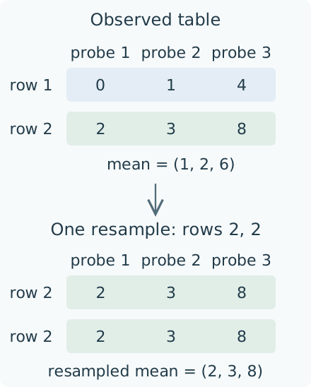
One possible resample of the two-row table. Repeating row 2 repeats all three of its values; choosing a separate row at each column would lose the observed relations between probes.
Let $\overline X^{*(b)}$ denote the mean of resample $b$. For a pointwise band, the algorithm retains $|\overline X^{*(b)}_j-\overline X_j|$ at each probe. For a simultaneous band it instead retains
\[D_b=\max_j |\overline X^{*(b)}_j-\overline X_j|.\]
Given $B$ resamples and requested level $\ell$, it sorts these deviations and uses the value in position $\lceil B\ell\rceil$ as a symmetric half-width around the observed mean. The simultaneous calculation uses one common half-width in the observable's units. There is no division by an estimated standard error, which is the meaning of nonstudentized here. A private pseudorandom generator, Xoshiro, uses the supplied seed and leaves the caller's random sequence unchanged.
This bootstrap approximates sampling uncertainty; it does not supply Hoeffding's finite sample guarantee. In a constant sample, for example, every resampled mean is identical and the band has width zero, although the unknown population need not be constant. At least two complete rows and an IID sampling declaration are required, but these checks cannot establish that the observations are independent. Dependent subjects or probes selected after looking at the data need an appropriate statistical method and justification.
García-Redondo, Monod and Wang's Confidence Bands for Multiparameter Persistence Landscapes develops a functional statistical theory for a specified multiparameter landscape and sampling model. It provides related background for mean inference. The implementation here operates on a finite vector of declared observables; arbitrary sampled slice landscapes do not inherit that paper's continuous-domain conclusion.
Drawing and selection consume prepared results
Featurizers owns the numerical calculation. Visualization receives its prepared summary, so selecting a probe or replicate does not rerun the bootstrap or change its seed. For one coordinate axis, the figure shows the sampled mean and band alongside a selected replicate and, when retained, its ordinary diagram. Connecting lines guide the eye between probes. For two axes, the picture preserves nonuniform physical coordinates and masks missing values. Mean and replicate values share a scale in the same units; frequency has a separate scale from zero to one.
The guide's prepared views follow individual rows through one descriptive summary and compare two thresholds on the same frequency scale. Their hand chosen intervals make the selected values checkable without introducing a sampling claim. Changing a browser choice selects one of those prepared figures; it does not rerun a summary or draw a new sample.
A selected observation retains its original coordinates and value beside the numerical summary. Optional source figures follow the supplied replicate IDs. The caller establishes those associations; the display does not prove a new correspondence between the objects. Before a live selection is accepted, a candidate snapshot is prepared. Invalid input leaves the previous snapshot visible. Linked viewers receive the accepted selection, and closing a session releases its inputs and listeners while retaining the final static snapshot. Inspection sessions explains these shared operations.
Costs and domain boundaries
For $n$ observations at $p$ probes, the input table stores $O(np)$ values and the summary stores $O(p)$. Sorting each column for empirical quantiles costs $O(pn\log n)$. With $B$ resamples, bootstrap arithmetic costs $O(Bnp)$; retained deviations use $O(Bp)$ space for pointwise bands or $O(B)$ for simultaneous bands. Construction, diagram evaluation, resampling and drawing each have explicit budgets. Exceeding one rejects the request rather than truncating the observations. No pairwise diagram distances are computed in this process.
A drawn strip between probes may look continuous, but the statistical domain remains finite. Extending a bound to intermediate parameters requires a regularity assumption and an estimate of the error from sampling. For example, a Betti count can jump at a birth, so a landscape's continuity estimate cannot be transferred to it merely because both are plotted on the same grid.
The arithmetic is numerical. Known bounds are converted outward to Float64 and their original declarations are retained. Endpoint rounding is adjusted outward so that a positive interval does not disappear through drawing precision. These guards address conversion and endpoint rounding; they do not turn every floating point reduction into an exact arithmetic certificate.