From a point cloud to comparisons and features
Download the executed notebook · Build and environment record
Moving one point changes the times at which connected components merge. We will use three points on a line to predict that change, compute the two barcodes, and compare numerical descriptions of them. The example is small enough that we can follow the answers back to the distances between the points.
You will need Julia, the latest version of TamerOp and CairoMakie in the notebook's environment; the installation page explains the setup. Degree zero homology records connected components. We use the default field with two elements throughout. After the comparison, we will save one diagram together with retained cocycle data and recover it from the file.
import TamerOp as OP
import CairoMakie
Three points and two merges
Put three points at 0, 2 and 5 on a line. A Vietoris–Rips filtration joins a pair when its distance is at most the parameter, and adds a simplex when all its edges are present. The parameter is therefore a diameter threshold, rather than the radius of a ball around each point.
At threshold zero the three points are separate components. At two the first two join, and at three the last point joins them. In degree zero we expect finite intervals [0,2) and [0,3), and one essential interval [0,infinity). The finite intervals include birth and exclude death; the essential interval records a component that survives at every later threshold.
Moving the last point to 6 changes the second merge to four. We keep the filtration rule, degree and coefficient field fixed so this change in the point position is the only change in the problem. Edges suffice to compute connected components, so max_dim=1 retains every dimension we need.
positions = [0.0, 2.0, 5.0]
changed_positions = [0.0, 2.0, 6.0]
cloud = OP.PointCloud([[x] for x in positions])
changed_cloud = OP.PointCloud([[x] for x in changed_positions])
filtration = OP.RipsFiltration(max_dim=1)
RipsFiltration
  kind: rips
  arity: 1
  key_params: (max_dim = 1, nn_backend = :auto, nn_approx_candidates = 0)
  construction_mode: (sparsify = :none, collapse = :none, output_stage = :encoding_result)
cloud_figure = CairoMakie.Figure(size=(500, 260), fontsize=18)
cloud_axis = CairoMakie.Axis(cloud_figure[1, 1]; xlabel="Position on the line",
yticks=([1, 2], ["Original", "Moved point"]), xticks=0:6,
limits=(-0.4, 6.4, 0.5, 2.5), ygridvisible=false)
CairoMakie.scatter!(cloud_axis, positions, fill(1, 3); color=:steelblue, markersize=14)
CairoMakie.scatter!(cloud_axis, changed_positions, fill(2, 3); color=:darkorange, markersize=14)
cloud_figure
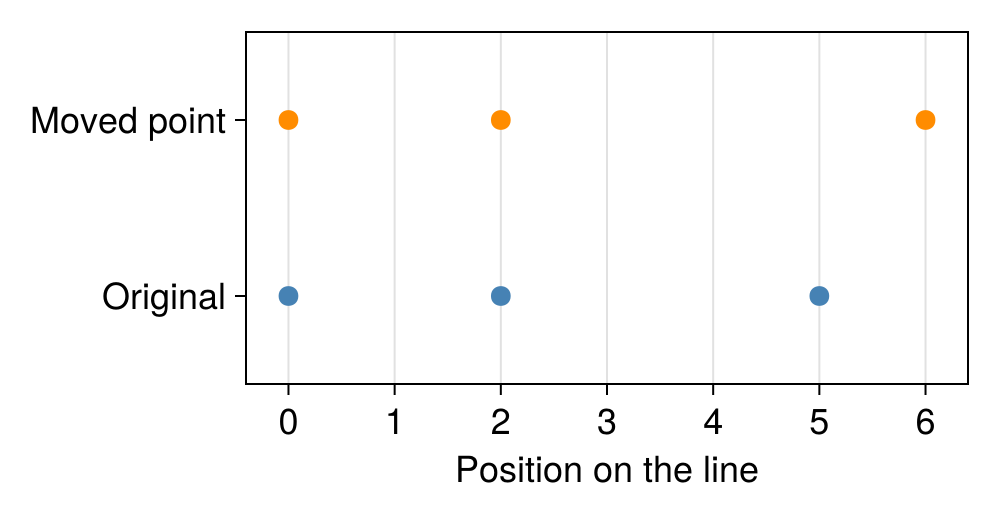
We request cocycles=true for the original cloud because we will later save and recover a degree zero cocycle. A cocycle assigns values to vertices that agree across every active edge, so it is constant on each component. Retaining these values costs additional work; the interval comparisons and features below do not need them. This request does not retain a full geometric source complex.
diagram = OP.persistence_diagram(cloud, filtration; max_homology_dim=0, cocycles=true)
changed = OP.persistence_diagram(changed_cloud, filtration; max_homology_dim=0)
OP.finite_intervals(diagram; dim=0)
2-element Vector{Tuple{Float64, Float64}}:
 (0.0, 2.0)
 (0.0, 3.0)
@assert sort(OP.finite_intervals(diagram; dim=0)) == [(0.0, 2.0), (0.0, 3.0)]
@assert sort(OP.finite_intervals(changed; dim=0)) == [(0.0, 2.0), (0.0, 4.0)]
@assert OP.essential_births(diagram; dim=0) == [0.0]
summary = OP.describe(diagram)
(finite=summary.finite_counts, essential=summary.essential_counts,
cocycles_retained=summary.cocycles_available)
(finite = (2,), essential = (1,), cocycles_retained = true)The first barcode records mergers at two and three; the second moves only the latter endpoint to four. An arrow marks the essential interval in each. We use the same display window so the shift in an endpoint has the same length in both pictures.
All three vertices are born at zero. Choosing which vertex labels the surviving component requires a tie convention, so the endpoints alone do not identify a particular source vertex.
OP.visualize(diagram; kind=:barcode, dim=0, window=(0, 5))
![Degree-zero persistence for the original cloud: finite intervals [0,2) and [0,3), and one essential interval born at zero. The rightward arrow records its infinite endpoint.](ordinary_analysis_files/ordinary_analysis_9_0.png)
OP.visualize(changed; kind=:barcode, dim=0, window=(0, 5))
![After moving the last point, the finite degree zero intervals are [0,2) and [0,4). The essential interval is unchanged. The display uses the same window as the original cloud.](ordinary_analysis_files/ordinary_analysis_10_0.png)
Compare the same degree
To compare barcodes, we match intervals while allowing an interval to be matched to the diagonal, which amounts to omitting it at a cost of half its lifetime. With the default q=Inf, the cost of matching two finite intervals is the larger of the differences between their births and deaths. The bottleneck distance minimizes the largest matching cost. The Wasserstein distance with p=2 minimizes the square root of the sum of squared costs.
Here the natural matching leaves [0,2) unchanged and matches [0,3) to [0,4) at cost one. No matching has smaller bottleneck cost: the interval ending at four must either match a finite interval with death at most three or pay two to match the diagonal. This proves that both distances below are one. The identical essential intervals match at cost zero; unequal essential counts would instead give infinity under the default convention.
The matching compares interval endpoints. To relate cells or chains from two source complexes, we would need additional maps between those complexes.
bottleneck = OP.bottleneck_distance(diagram, changed; dim=0)
wasserstein = OP.wasserstein_distance(diagram, changed; dim=0, p=2)
@assert bottleneck == wasserstein == 1.0
(bottleneck=bottleneck, wasserstein=wasserstein)
(bottleneck = 1.0, wasserstein = 1.0)Choose how essential intervals enter the features
Landscapes, persistence images and lifetime summaries use finite intervals. We choose essential=:drop to study the mergers, omitting the component that survives forever. This choice affects the feature calculation and leaves the original diagram intact. analysis_barcode shows the intervals in the increasing parameter coordinate used by those calculations.
Another choice is essential=:cap, essential_cap=6, which replaces the infinite endpoint by six for this analysis. The cap describes a chosen observation convention. It is not a death computed from the filtration.
OP.analysis_barcode(diagram; dim=0, essential=:drop)
2-element Vector{Tuple{Rational{BigInt}, Rational{BigInt}}}:
 (0, 2)
 (0, 3)
capped = OP.analysis_barcode(diagram; dim=0, essential=:cap, essential_cap=6)
@assert sort(capped) == [(0, 2), (0, 3), (0, 6)]
capped
3-element Vector{Tuple{Rational{BigInt}, Rational{BigInt}}}:
 (0, 2)
 (0, 3)
 (0, 6)
Landscapes on a common grid
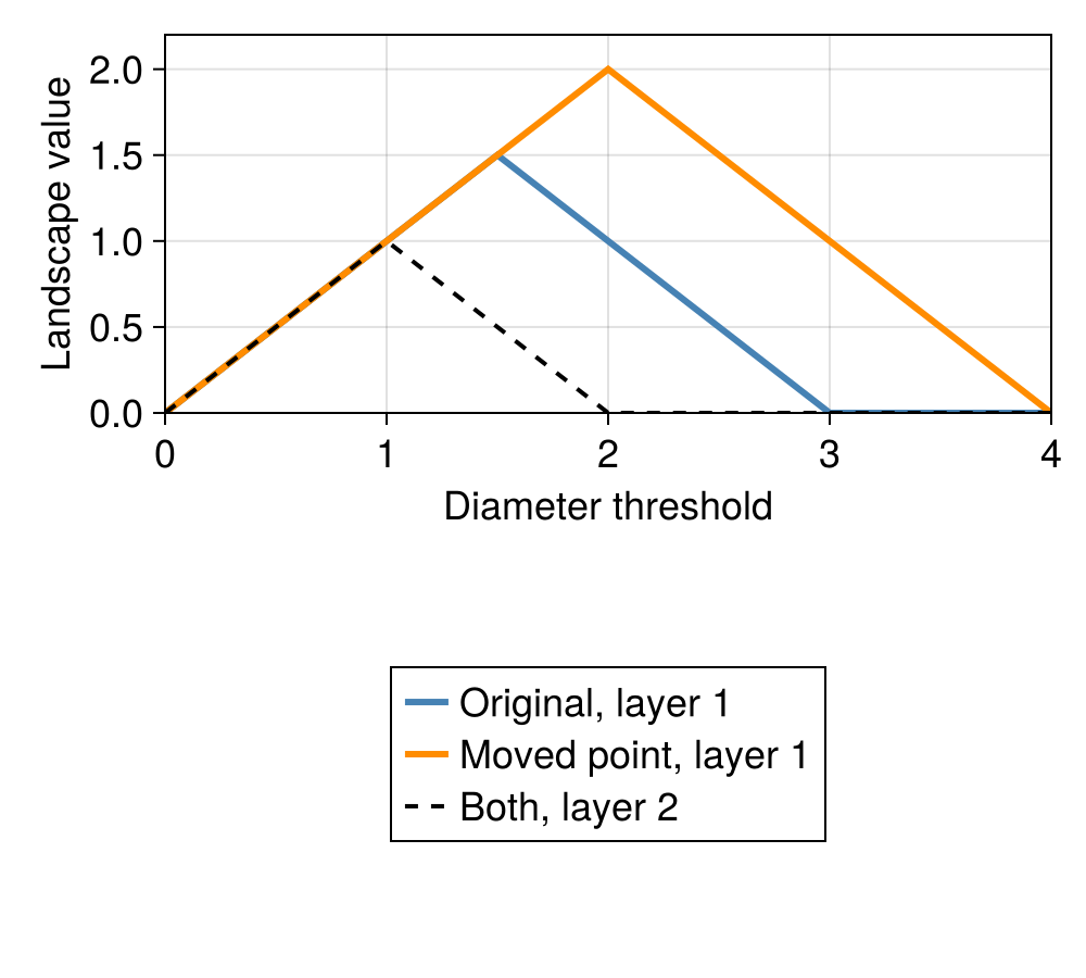
An interval with birth $b$ and death $d$ contributes a tent of height $\min(t-b,d-t)$ for $b\leq t\leq d$, and zero outside. At each $t$, the first persistence landscape layer is the largest tent value, the second is the next largest, and so on. We sample both clouds on the same grid so an array entry refers to the same parameter in either result.
At threshold one, both original intervals contribute height one. We can check the two landscape entries at that grid point before looking at their graphs.
grid = 0.0:0.5:4.0
landscape = OP.persistence_landscape(diagram; dim=0, essential=:drop, tgrid=grid, kmax=2)
changed_landscape = OP.persistence_landscape(changed; dim=0, essential=:drop, tgrid=grid, kmax=2)
@assert OP.Advanced.landscape_values(landscape)[:, 3] == [1.0, 1.0]
OP.Advanced.landscape_values(landscape)
2×9 Matrix{Float64}:
 0.0  0.5  1.0  1.5  1.0  0.5  0.0  0.0  0.0
 0.0  0.5  1.0  0.5  0.0  0.0  0.0  0.0  0.0
Moving the point lengthens [0,3) to [0,4), so that interval's tent becomes wider and its peak rises from 1.5 to two. In this example it stays at least as high as the tent from [0,2), so it supplies the first layer. The unchanged tent supplies the second layer in both clouds.
Our grid contains the corners of these particular tents, including their peaks. Joining consecutive samples therefore recovers the full piecewise linear graphs here. For a different barcode, a coarser grid can miss a corner.
landscape_figure = CairoMakie.Figure(size=(500, 450), fontsize=18)
landscape_axis = CairoMakie.Axis(landscape_figure[1, 1];
    xlabel="Diameter threshold", ylabel="Landscape value", xticks=0:4,
    limits=(0, 4, 0, 2.2))
CairoMakie.lines!(landscape_axis, grid, OP.Advanced.landscape_values(landscape)[1, :];
    label="Original, layer 1", color=:steelblue, linewidth=3)
CairoMakie.lines!(landscape_axis, grid, OP.Advanced.landscape_values(changed_landscape)[1, :];
    label="Moved point, layer 1", color=:darkorange, linewidth=3)
CairoMakie.lines!(landscape_axis, grid, OP.Advanced.landscape_values(landscape)[2, :];
    label="Both, layer 2", color=:black, linestyle=:dash, linewidth=2)
CairoMakie.Legend(landscape_figure[2, 1], landscape_axis; labelsize=18, tellwidth=false)
landscape_figure
A persistence silhouette gives another view of the same tents by taking a weighted average instead of sorting their heights into layers. With the default lifetime weights two and three, its value at threshold one is (2*1 + 3*1)/(2+3) = 1. At threshold two the shorter tent has reached zero and the longer one has height one, giving 3/5.
silhouette = OP.persistence_silhouette(diagram; dim=0, essential=:drop, tgrid=grid)
@assert silhouette[3] == 1.0 && silhouette[5] == 0.6
silhouette
9-element Vector{Float64}:
 0.0
 0.5
 1.0
 1.1
 0.6
 0.3
 0.0
 0.0
 0.0
A persistence image and two scalar summaries
A persistence image places a Gaussian at each point whose coordinates are birth and lifetime, then samples their weighted sum on a rectangular grid. Here both births are zero and the lifetimes are two and three. The default weights are those lifetimes, so the longer interval contributes more.
The small matrix below has lifetime coordinates along its rows and birth coordinates along its columns. Its entries are sampled Gaussian values, rather than integrals over pixels. Comparing such matrices requires the same coordinates, grid, bandwidth, weighting and normalization; otherwise an entry could change because we changed the measurement itself.
image = OP.persistence_image(diagram; dim=0, essential=:drop,
    xgrid=[0.0, 1.0, 2.0], ygrid=[0.0, 1.0, 2.0, 3.0, 4.0], sigma=0.5)
OP.Advanced.image_values(image)
5×3 Matrix{Float64}:
 0.000670971  9.0806e-5  2.25086e-7
 0.271677     0.0367675  9.11375e-5
 2.40601      0.325617   0.000807125
 3.27067      0.442637   0.00109719
 0.406677     0.0550377  0.000136425
The total persistence is the sum of lifetimes, 2+3=5. Persistent entropy measures how evenly that sum is distributed among the intervals. Their shares are 2/5 and 3/5, so unnormalized entropy is -(2/5)log(2/5)-(3/5)log(3/5). The normalized default divides by the logarithm of the number of intervals; we turn off that normalization to check the displayed formula directly.
statistics = OP.barcode_summary(diagram; dim=0, essential=:drop)
entropy = OP.barcode_entropy(diagram; dim=0, essential=:drop, normalize=false)
@assert statistics.n_intervals == 2 && statistics.total_persistence == 5.0
@assert isapprox(entropy, -(2/5)*log(2/5)-(3/5)*log(3/5))
(statistics=statistics, entropy=entropy)
(statistics = (n_intervals = 2, total_persistence = 5.0, max_persistence = 3.0, mean_persistence = 2.5, l2_persistence = 3.605551275463989, entropy = 0.9709505944546688), entropy = 0.6730116670092565)Save and recover the diagram
A feature vector has already discarded information from the diagram. If we want to revisit the intervals, coefficient field, filtration order or retained cocycles, we can save the diagram itself. We use a temporary folder here so rerunning the notebook does not overwrite an earlier analysis. In your own work, replace it with the destination where you want to keep the result.
result_folder = mktempdir()
result_path = joinpath(result_folder, "ordinary-diagram.json")
OP.save_persistence_diagram_json(result_path, diagram)
restored = OP.load_persistence_diagram_json(result_path)
@assert OP.Advanced.check_persistence_diagram_json(result_path).valid
@assert OP.finite_intervals(restored; dim=0) == OP.finite_intervals(diagram; dim=0)
@assert OP.essential_births(restored; dim=0) == OP.essential_births(diagram; dim=0)
@assert OP.Advanced.field(restored) == OP.Advanced.field(diagram)
@assert OP.Advanced.filtration_order(restored) == OP.Advanced.filtration_order(diagram)
@assert OP.bottleneck_distance(restored, diagram; dim=0) == 0.0
OP.inspect_json(result_path)
JSONArtifactSummary
  path: "/tmp/jl_Ot32mH/ordinary-diagram.json"
  kind: "PersistenceDiagram"
  schema_version: 2
  field: "Fp"
  field_characteristic: 2
  order: "sublevel"
  finite_counts: [2]
  essential_counts: [1]
  representatives_available: false
  cocycles_available: true
  profile_hint: :compact
  size_bytes: 18185
At threshold four all three original points are connected. A degree zero cocycle on the essential component is constant across its vertices. We recover the retained cocycle at that threshold and compare it with the original record, including the original point indices.
The file in this example contains intervals and retained cocycle data, not the full source cloud or a retained geometric complex. Loading validates the stored structure; the equality check below confirms that the cocycle record survived this round trip.
original_cocycle = OP.Advanced.persistence_cocycle(diagram; dim=0, kind=:essential, scale=4)
restored_cocycle = OP.Advanced.persistence_cocycle(restored; dim=0, kind=:essential, scale=4)
@assert restored_cocycle == original_cocycle
restored_cocycle.source_vertices
((1,), (2,), (3,))Try one change
What should the total persistence become if we include the essential interval with a cap at six? The two computed finite lifetimes remain two and three, and our chosen cap contributes six. The following cell checks their sum.
capped_statistics = OP.barcode_summary(diagram; dim=0, essential=:cap, essential_cap=6)
@assert capped_statistics.total_persistence == 11.0
capped_statistics
(n_intervals = 3, total_persistence = 11.0, max_persistence = 6.0, mean_persistence = 3.6666666666666665, l2_persistence = 7.0, entropy = 0.9056185178648963)Coordinates for another dataset
The point clouds here use sublevel thresholds in their original units. For another dataset, origin and positive scale transform those grades to (grade-origin)/scale. Superlevel diagrams instead use (origin-grade)/scale, so both analyses advance in an increasing coordinate. Supply any essential cap in original grade units, and supply numerical grids in the transformed coordinate.
A common origin and scale can keep large nearby grades distinguishable when converting them to floating point for sampled features. Use the same transformation for results whose physical parameter you intend to compare. Exact interval data remain exact in the diagram, while these distances and sampled features are numerical outputs.
For the three points, moving the final point delayed one merge by one unit. We saw that same change in a barcode endpoint, a comparison distance and the first landscape layer, then retained the diagram so we could return to its cocycle data. The ordinary persistence guide explains further construction choices, and the source cells guide follows representatives back to retained geometry. The next cell removes the temporary folder created for this example.
rm(result_folder; recursive=true)