Composing and sharing mathematical figures
Download the executed notebook · Build and environment record
Suppose we have drawn the dimensions of a module and would like to show where those dimensions change. Placing the two pictures together lets us follow a number in one view back to the calculation that produced it. We need to keep the coordinates and scales consistent, and explain what any connecting arrow means.
We will begin with two overlapping squares, using their dimension table to build a picture of signed changes. Then we will connect a cycle in an image to its persistence interval. This second connection comes from retained computational data; a later optional example shows how to add an explanation of our own. The distinction matters when a reader tries to infer a mathematical relationship from a figure.
The examples use TamerOp and CairoMakie; see the installation page for setup. A matrix and a barcode are enough to begin. The signed summaries lesson and source cells lesson develop the underlying objects further. On a narrow screen, scroll across a figure to read its labels, or select it to open the full image.
import TamerOp as OP
using CairoMakie
A = OP.AdvancedTamerOp.AdvancedPut changes in dimension back in context
Consider the direct sum of two modules supported on the squares $[0,2)^2$ and $[1,3)^2$. Each contributes a one dimensional vector space on its square, with identity maps between comparable points there and zero spaces elsewhere. The dimension of their direct sum is therefore two where the squares overlap, one where exactly one is present, and zero outside both. We supply these dimensions by their formulas and sample them on the following grid.
A signed atom is a point carrying a positive or negative weight. To describe the first square, place weight $+1$ at $(0,0)$, weight $-1$ at $(2,0)$ and $(0,2)$, and weight $+1$ at $(2,2)$. At a query $(x,y)$, sum the weights of all atoms whose two coordinates are at most $x$ and $y$. Inside the square only the first atom contributes. Crossing one upper boundary adds a negative weight and returns the sum to zero; beyond both boundaries the last positive weight corrects for having subtracted twice.
The second square contributes the same four weights translated by $(1,1)$. Their sum is the point signed measure of the dimension table. Negative weights describe cancellation in this cumulative sum; all the dimensions we reconstruct remain nonnegative.
xs = [-1, 0, 1, 2, 3, 4]
ys = [-1, 0, 1, 2, 3, 4]
dimensions = [Int(0 <= x < 2 && 0 <= y < 2) +
              Int(1 <= x < 3 && 1 <= y < 3) for x in xs, y in ys]
atoms = OP.SignedMeasures.point_signed_measure(dimensions, (xs, ys))
@assert dimensions[3, 3] == 2
OP.describe(atoms)
(kind = :point_signed_measure, ambient_dimension = 2, axis_lengths = (6, 6), nterms = 8, positive_terms = 4, negative_terms = 4, total_mass = 0, total_variation = 8, largest_terms = [(index = (2, 2), point = (0, 0), weight = 1), (index = (4, 2), point = (2, 0), weight = -1), (index = (3, 3), point = (1, 1), weight = 1), (index = (5, 3), point = (3, 1), weight = -1), (index = (2, 4), point = (0, 2), weight = -1)])Before drawing, we can check this description against every entry in the table. The loop below sums the weights below each grid point and compares the result with the supplied dimension. For example, at $(1,1)$ both lower corners contribute, giving two. At $(2,1)$ the first square has ended and its two contributing weights cancel, leaving one from the second square.
The VisualContext records which parameter domain, units and data the panels refer to. We give the background and the atoms the same context because we calculated them from the same table. The library checks these declarations when combining views; the cumulative calculation below establishes the particular relationship we are drawing.
context = OP.VisualContext(domain="two-square parameter plane",
    units=("first parameter", "second parameter"), provenance="two square support formulas")
for (i, x) in enumerate(xs), (j, y) in enumerate(ys)
    reconstructed = sum((w for (p, w) in zip(OP.SignedMeasures.points(atoms),
        OP.SignedMeasures.weights(atoms)) if p[1] <= x && p[2] <= y); init=0)
    @assert reconstructed == dimensions[i, j]
end
background = OP.visual_panel(permutedims(dimensions); x=xs, y=ys,
    quantity="dimension", context, title="Dimensions of two squares")
OP.visualize(background)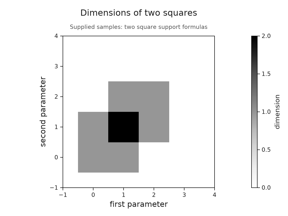
The table was constructed with $x$ as its first index, while rows in the plotted matrix follow the vertical coordinate $y$. permutedims puts the values into that drawing convention. The gray cells are centred on the sample coordinates. Their edges consequently do not draw the exact boundaries of the two square modules; those boundaries are specified by the formulas above.
We can now place the signed atoms over this background. The names dimensions and changes retain the identities of the two layers. Their order puts the atoms in front of the shading, and the common viewing window keeps the zero region visible around them.
signed = OP.visual_panel(atoms; kind=:signed_atoms, context,
    limits=(x=(-1, 4), y=(-1, 4)))
overlay = OP.overlay_visuals((dimensions=background, changes=signed);
    title="Dimension and its signed changes")
OP.visualize(overlay)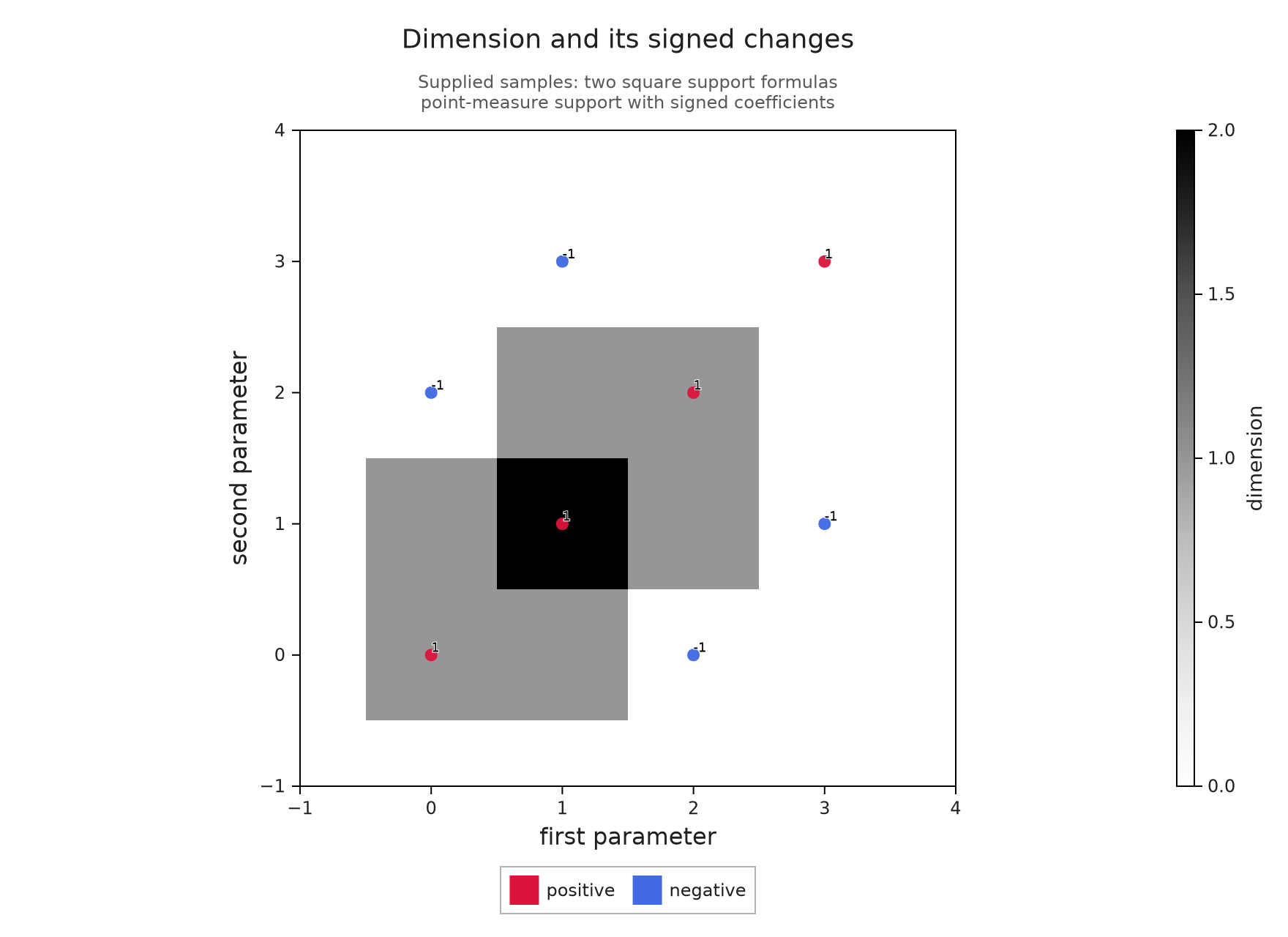
At the grid point $(1,1)$, the darkest shade and the two contributing positive atoms give two ways of reading the dimension two. At $(2,1)$, the negative atom at $(2,0)$ cancels the first square's contribution. The colorbar measures dimensions, while the red and blue markers distinguish positive and negative weights; their numerical labels let us read the signs without relying on color.
To point out the overlap, we add a rectangular highlight whose corners are given in parameter coordinates. This is an explanation we supply. Its dashed outline and legend distinguish it from the computed weights, and its bounds mark the overlap in the formulas rather than the edges of the shaded sample cells.
overlap_note = OP.VisualAnnotation(
    OP.VisualAnchor(:summary; point=(1, 1)),
    OP.VisualAnchor(:summary; point=(2, 2));
    kind=:highlight, label="Both squares contribute")
summary_figure = OP.compose_visuals((summary=overlay,);
    annotations=(overlap_note,), title="Read the dimensions and the changes together")
OP.visualize(summary_figure)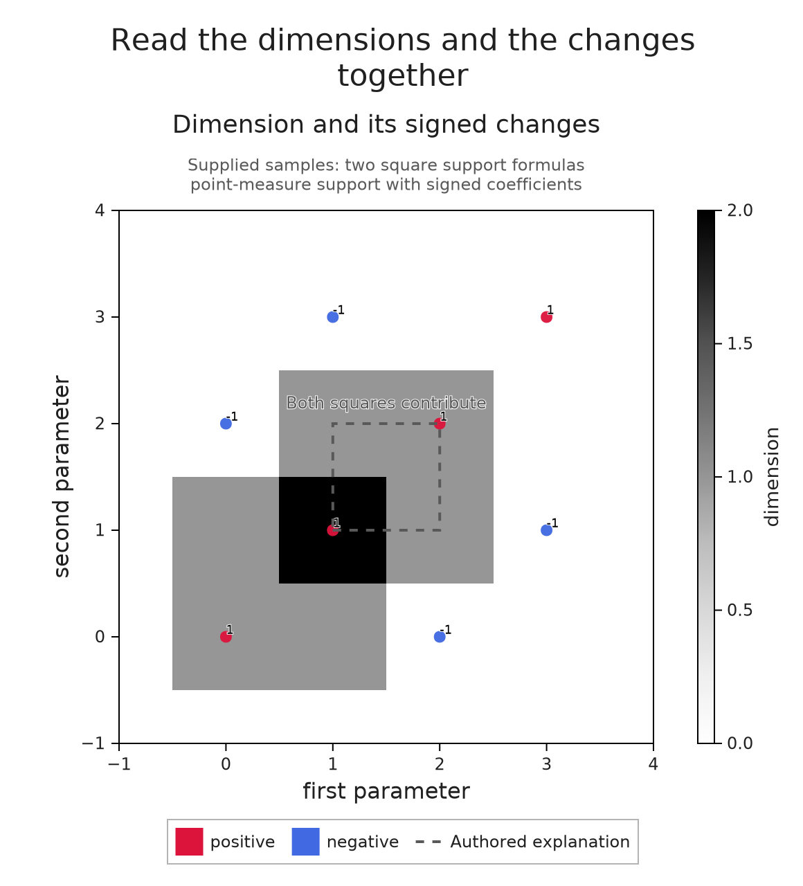
Compare with one scale
Suppose a second table contains twice the dimensions. If each panel chooses its own color range, its largest value can receive the same shade even though one maximum is two and the other is four. Linking the color ranges makes both panels use zero through four, so we can compare their numerical values by looking at their shades.
The tables have different data descriptions, which we identify in comparison. Their parameter coordinates still agree. We link the axes as well as the colors, and use columns=1 to put the two panels one above the other. This changes the arrangement while preserving the common scales and the supplied values.
double_context = OP.VisualContext(domain="two-square parameter plane",
    units=context.units, provenance="twice the two-square dimension table")
doubled = OP.visual_panel(2 .* permutedims(dimensions); x=xs, y=ys,
    quantity="dimension", context=double_context, title="Twice the dimension table")
comparison = OP.compose_visuals((original=background, doubled=doubled);
    link_axes=((:original, :doubled),), link_colors=((:original, :doubled),),
    columns=1, comparison="Original table and its doubled values",
    title="Comparing dimensions on a common scale")
OP.visualize(comparison)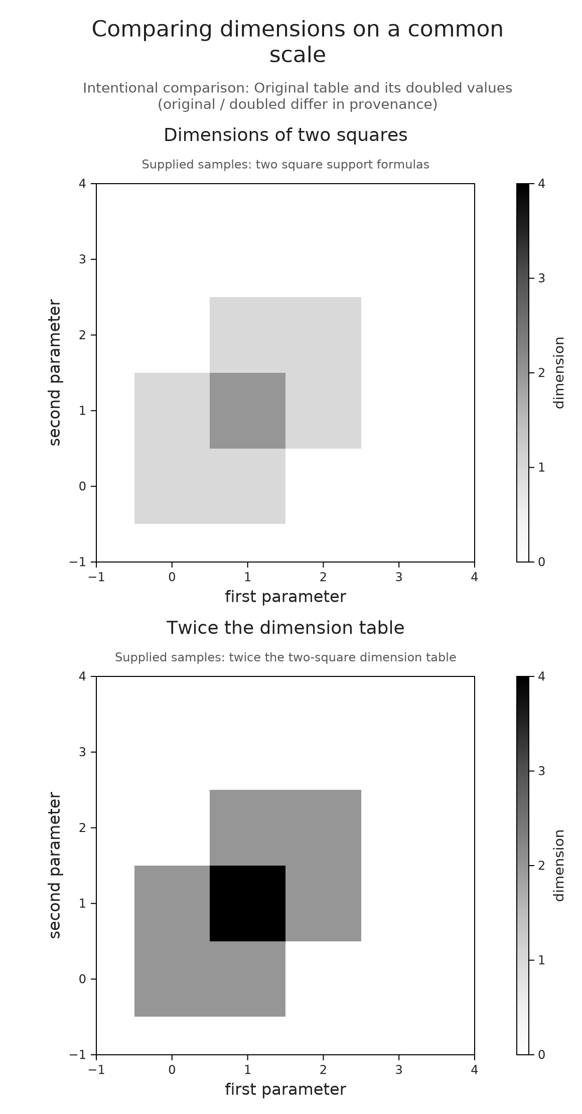
The overlap in the original table is now halfway up the shared scale, while its doubled value reaches four. We can read that difference because a shade has the same meaning in both panels. Sharing these scales makes a numerical comparison possible; it does not identify vector spaces or homology classes between the two constructions.
The declarations also prevent accidental comparisons. For example, changing one panel's first unit to millimeters creates a disagreement. Linking the panels without a comparison explanation is then rejected. Supplying an explanation permits the juxtaposition and records the disagreement, but it performs no unit conversion. The composition reference lists the compatibility conditions.
Connect a class to the source that represents it
We can give a connecting arrow a more specific meaning when both ends come from the same computation. Take a $3\times3$ image whose outer eight squares enter at parameter zero and whose centre enters at five. Until five there is a hole; adding the centre fills it. In homology degree one this gives the interval $[0,5)$.
We retain the source cells and ask for a representative at parameter two. A cycle is a chain with zero boundary, and a representative cycle is one whose homology class is the requested element. Here the coefficients lie in $\mathbb F_2$, the field with two elements, so an edge either appears with coefficient one or is absent. The source cells lesson explains how this chain is recovered from the persistence calculation. Here A abbreviates OP.Advanced, which provides the representative query.
image = zeros(Int, 3, 3)
image[2, 2] = 5
diagram = OP.cubical_persistence(image; input=:top_cells,
    source=true, representatives=true)
representative = A.persistence_representative(diagram; dim=1, scale=2)
cycle = representative.source_cycle
@assert representative.interval == (0, 5)
OP.describe(cycle)
(kind = :source_chain, chain_kind = :cycle, dimension = 1, parameter = (2,), field = TamerOp.CoreModules.CoeffFields.PrimeField(2), cell_count = 24, support = 4, metadata = (correspondence = :verified_chain_map, certificate = :equal_grade_contraction, choice = :noncanonical_f2_column_reduction, equation = :checked_on_source, optimization = :none, interval = (0, 5), interval_kind = :finite, member = 1))The source panel draws the cycle on the original image cells. The barcode panel draws its interval, retaining the identity of the original interval even if several equal bars are grouped into one row. correspondence_annotation checks the source, field, parameter and coefficients against the representative retained by this diagram, then chooses endpoints in those two panels.
We arrange the panels in one column so each has more room in the article. The names source and barcode identify the panels for the connector regardless of this layout choice.
source = OP.visual_panel(cycle; title="A cycle around the missing center")
barcode = OP.visual_panel(diagram; kind=:barcode, dim=1)
connection = OP.correspondence_annotation(diagram, cycle;
    label="Represents this\ninterval", curve=0.40)
source_figure = OP.compose_visuals((source=source, barcode=barcode);
    annotations=(connection,), columns=1, title="A class and one of its representatives")
OP.visualize(source_figure)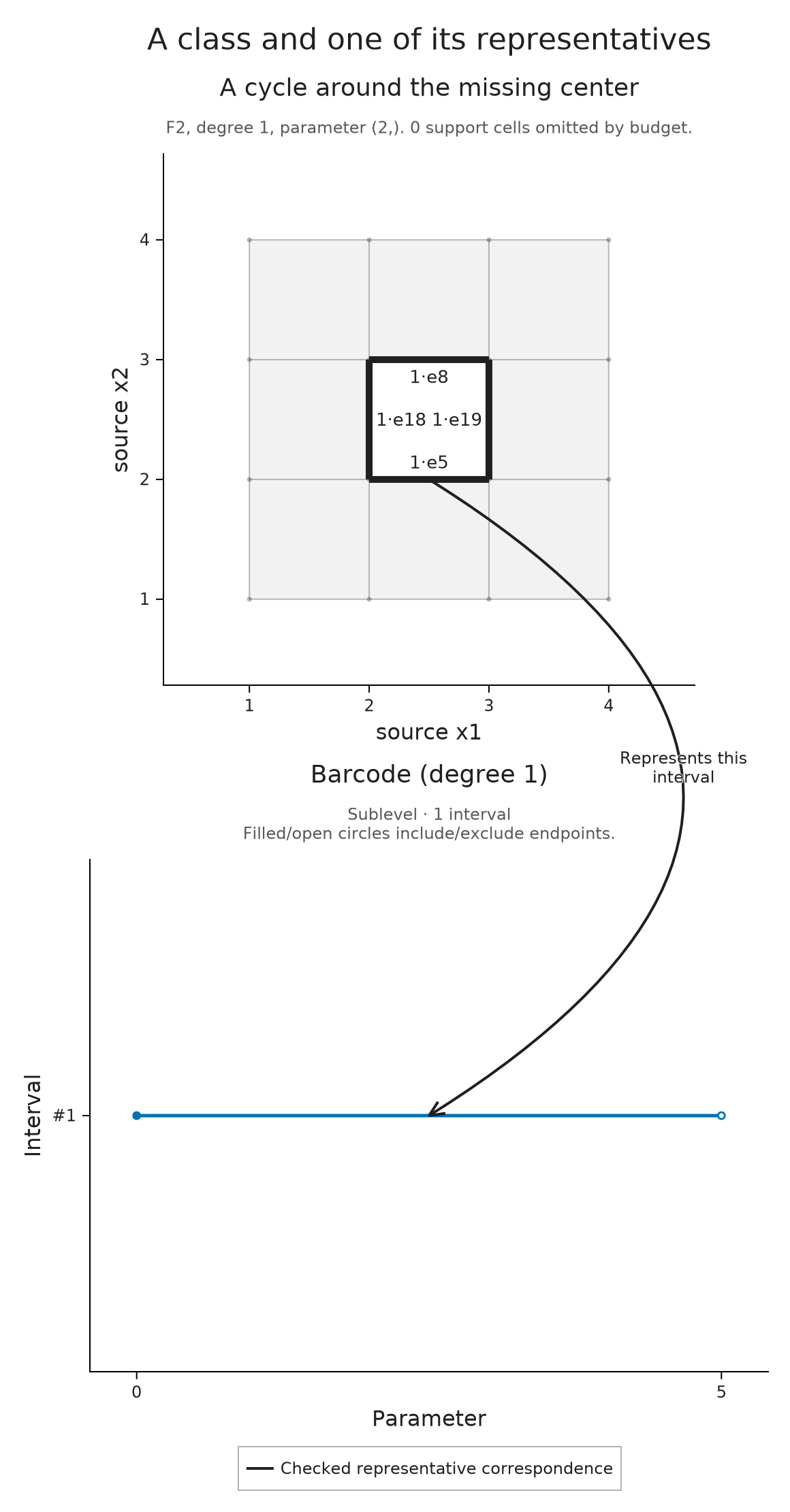
The solid arrow joins an edge of the displayed cycle to its interval. Its meaning comes from the check we just requested: this chain represents that interval's class at parameter two. The computation chooses a representative; it does not establish that this cycle is shortest or canonical, or that it belongs to a summand of a module with several parameters. The class remains alive at four, while five is excluded from the interval and cannot be used for this representative query.
Annotation endpoints refer to mathematical objects or data coordinates before the figure is laid out. Reordering the named panels or changing the figure size therefore keeps the arrow attached. If a drawing limit omits its chosen source cell or interval, composition rejects that missing endpoint. This is useful when making a smaller picture: we learn that part of the explanation would no longer be visible.
Optional: extend the interval to a second parameter
Relate source geometry to a parameter support
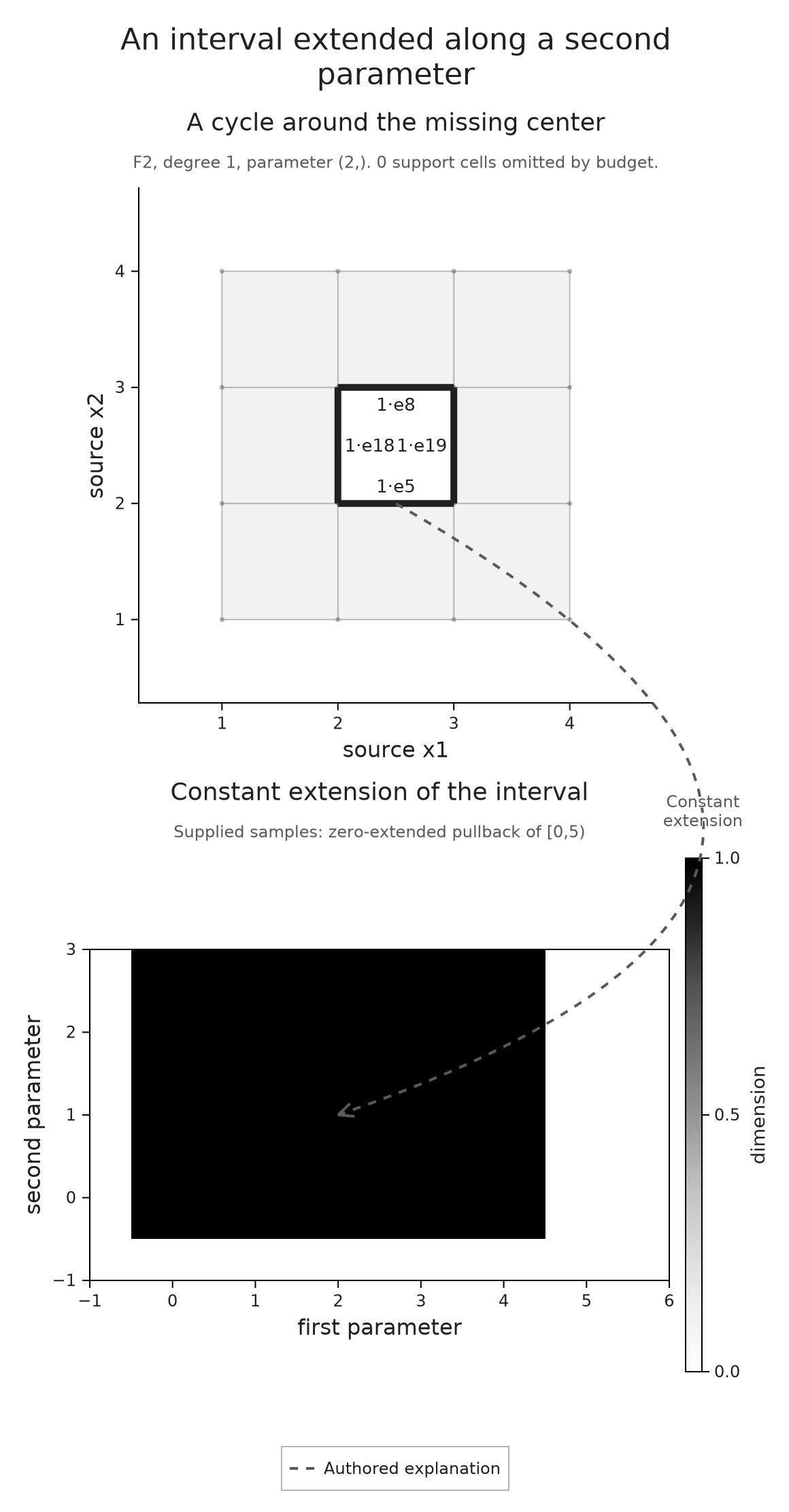
We can use the same source picture to explain a construction that we specify ourselves. Let $I$ be the interval module for $[0,5)$, and define a module on $\mathbb R\times[0,\infty)$ by assigning $I(r)$ to $(r,s)$. For a comparable pair, use the map from $I(r)$ to $I(r')$. This is the pullback along the projection $(r,s)\mapsto r$: the second coordinate leaves the interval unchanged. Extending by zero to the rest of the plane makes all spaces with $s<0$ zero. The resulting support is $[0,5)\times[0,\infty)$.
The shaded table below samples this declared module in a finite window. A dashed arrow connects the source cycle to a point of its support as an explanation of the construction. We have supplied this relationship; the library has not inferred a module decomposition from the image.
first_parameter = collect(-1:6)
second_parameter = collect(-1:3)
support_values = [Int(0 <= r < 5 && s >= 0) for s in second_parameter, r in first_parameter]
support_context = OP.VisualContext(domain="first and second parameter",
    units=("first parameter", "second parameter"), degree=1, provenance="zero-extended pullback of [0,5)")
support = OP.visual_panel(support_values; x=first_parameter, y=second_parameter,
    quantity="dimension", context=support_context, title="Constant extension of the interval")
support_note = OP.VisualAnnotation(connection.from,
    OP.VisualAnchor(:support; point=(2, 1));
    label="Constant\nextension", curve=0.55)
support_figure = OP.compose_visuals((source=source, support=support);
    annotations=(support_note,), columns=1, title="An interval extended along a second parameter")
OP.visualize(support_figure)
Optional: annotate an algebraic coefficient
Explain a coefficient without asserting another map
An annotation can follow a coefficient through an algebraic description. In the supplied matrix below, the first column is $g_1=u-v$. We draw a separate schematic marker for $g_1$ and connect it to the coefficient $-1$ in row $v$. The marker's position is chosen for the diagram; it is not a computed grade of a generator.
VisualAnchor identifies an endpoint of an annotation. The matrix endpoint uses its row and column to find the actual coefficient label, while the other endpoint selects the first point in the schematic. A dashed arrow records this authored explanation without asserting a further structure map.
matrix = A.VisualizationSpec(:presentation_fragment;
    title="A supplied presentation fragment",
    layers=A.AbstractVisualizationLayer[
        A.MatrixLayer(["1" "0"; "-1" "2"], ["u", "v"], ["g1", "g2"])],
    metadata=(panel_style=:matrix,))
generators = A.VisualizationSpec(:generator_schematic;
    title="Generator labels (schematic)",
    layers=A.AbstractVisualizationLayer[
        A.PointLayer([(0.0, 0.0), (1.0, 1.0)], :royalblue, 1.0, 12.0),
        A.TextLayer(["g1", "g2"], [(0.0, 0.2), (1.0, 1.2)], :black, 16.0)],
    axes=(xlabel="layout", ylabel="layout", xlimits=(-0.5, 1.5),
          ylimits=(-0.5, 1.5), aspect=:equal))
coefficient_note = OP.VisualAnnotation(
    OP.VisualAnchor(:matrix; target=(:matrix, 2, 1)),
    OP.VisualAnchor(:generators; target=(:layer, 1, 1));
    label="Coefficient -1 in g1", curve=-0.12)
algebra_figure = OP.compose_visuals((matrix=matrix, generators=generators);
    annotations=(coefficient_note,), columns=1, title="Keep the coefficient attached to its label")
OP.visualize(algebra_figure)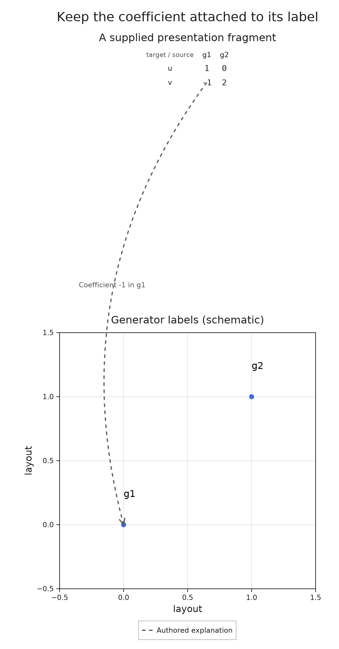
Optional: export the selected figure
We can save the current figure as PNG, SVG or PDF, or place its SVG inside a standalone HTML file. That HTML preserves one selected view and a text description of its annotations. It can be reopened with Julia closed and without network access. On a narrow screen its figure can be scrolled at the saved size, keeping the labels readable and the arrows attached to their endpoints.
The files go in tamerop_outputs/composed-figures under the current working directory. Rerunning the cell replaces these named examples; choose a different destination for a figure you want to keep separately. The links after the cell offer each format of the cycle and interval composition, so you can inspect the result without running the notebook.
output_directory = joinpath("tamerop_outputs", "composed-figures")
mkpath(output_directory)
exports = [OP.save_visual(output_directory, "cycle-connection", source_figure; format)
           for format in (:png, :svg, :pdf, :html)]
[(OP.export_format(result), basename(OP.export_path(result))) for result in exports]
4-element Vector{Tuple{Symbol, String}}:
(:png, "cycle-connection.png")
(:svg, "cycle-connection.svg")
(:pdf, "cycle-connection.pdf")
(:html, "cycle-connection.html")Open the cycle and interval composition
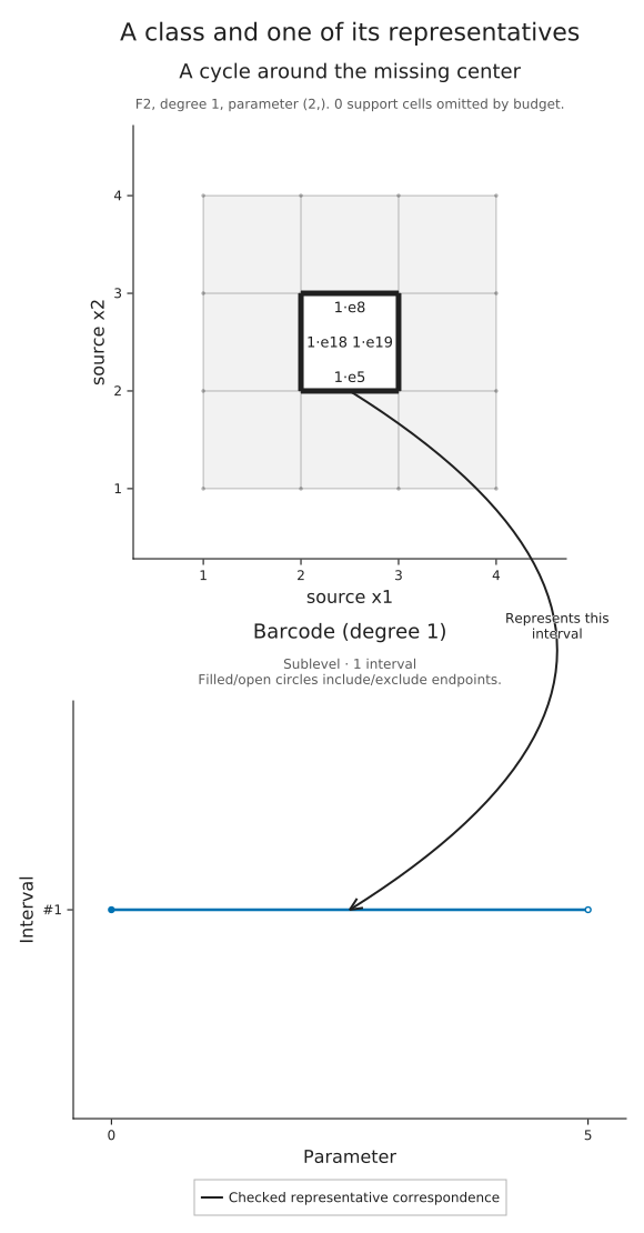
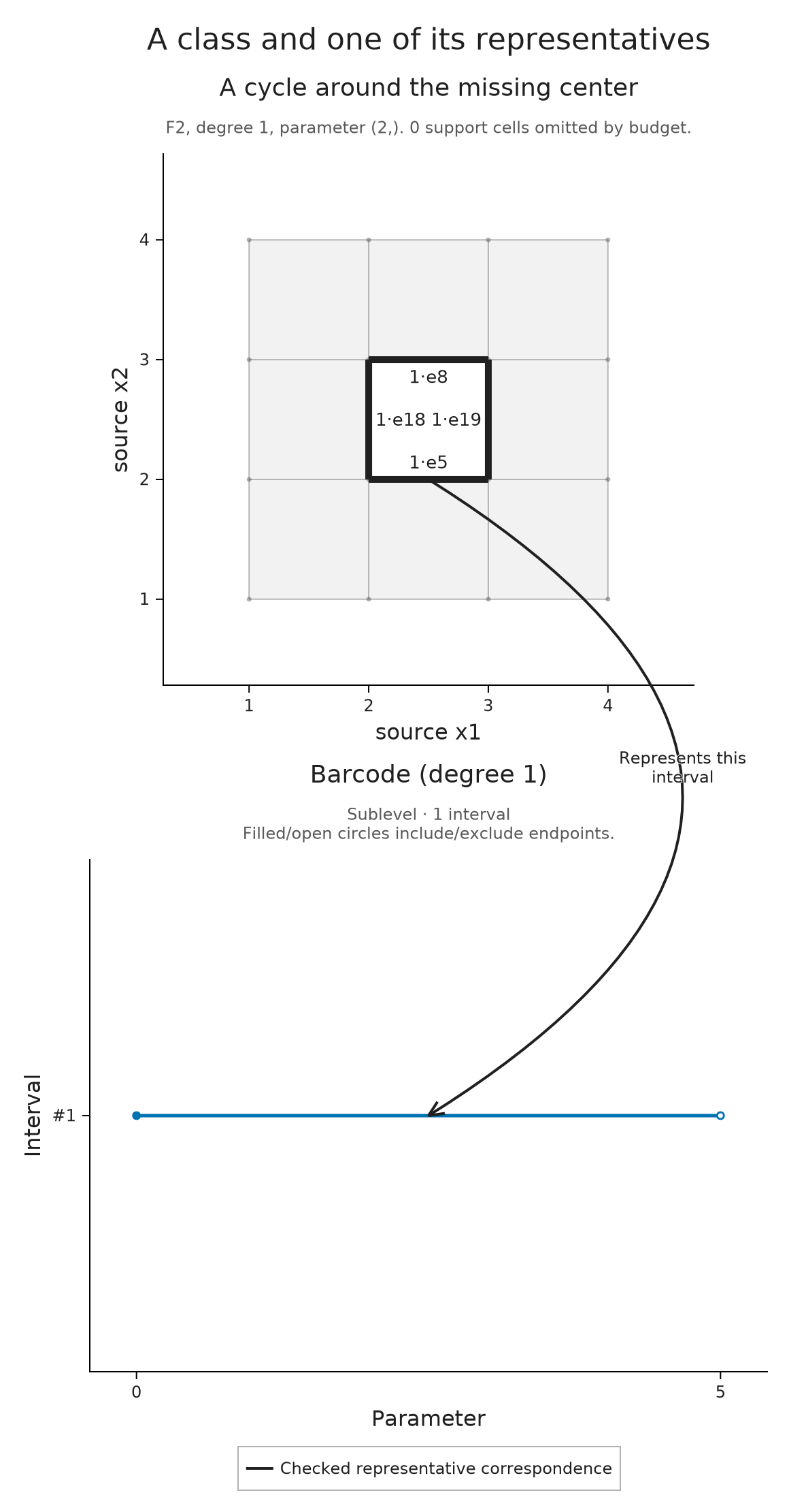
A grayscale export can use the same composition. It preserves the cycle, interval and checked connector while changing their appearance. The solid line and legend continue to explain the relationship without depending on color.
OP.visualize(source_figure; style=OP.VisualStyle(palette=:grayscale))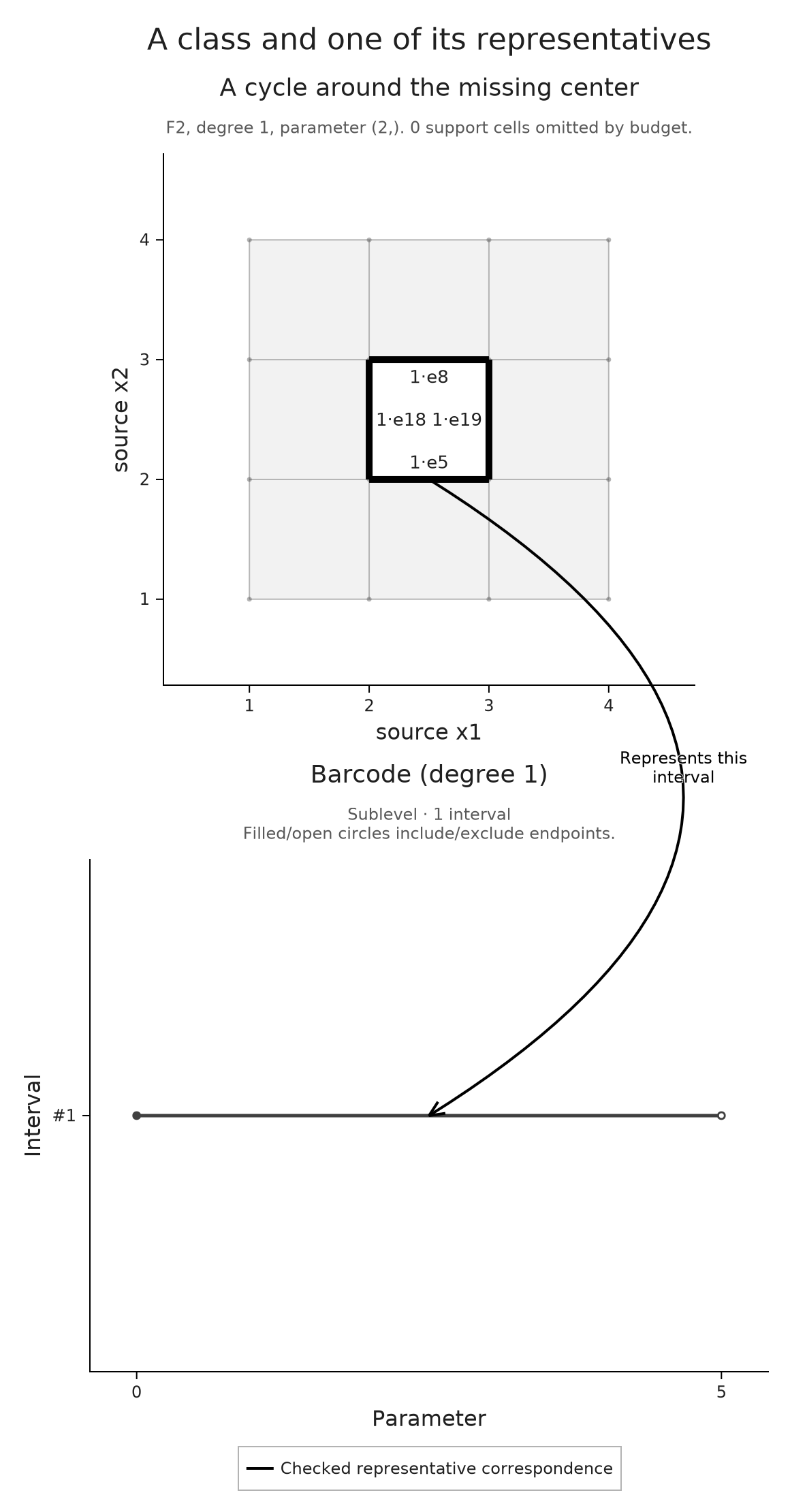
The saved composition preserves the choices we made for one figure. To keep several selections, reopen their exact readouts or resume queries in Julia, continue with Keeping a selected mathematical view, which develops the saved session workflow. To retain a mathematical object independently of its picture, use the integration and interchange guide.