Analyzing ensembles of persistence results
Download the executed notebook · Build and environment record
Suppose we compute persistence for several inputs and ask for a landscape value at the same parameter in each result. We can collect the answers, take their mean, and see how widely they vary. The same idea applies to the dimension of an encoded module at an original parameter value, even when different inputs use different finite encodings. What matters is that each answer comes from the same mathematical question.
An ensemble here is this collection of repeated observations, together with the coordinates and choices that let us compare them. We will begin with three intervals whose landscape values can be computed by hand, then query two finite modules on a common grid. These examples give us a way to read the figures before considering what additional assumptions are needed to infer a population mean.
Familiarity with ordinary persistence is enough for the first example. Install TamerOp and CairoMakie to execute the figures. WGLMakie is needed only for the optional live view.
import TamerOp as OP
using CairoMakie
A = OP.Advanced
V = OP.Visualization
CairoMakie.activate!()
Repeat the same observable
An observable is the numerical quantity we choose to measure. Take the intervals $[0,2)$, $[0,4)$ and $[0,6)$ in homological degree zero over $\mathbb F_2$. For a single finite interval $[b,d)$, its first persistence landscape is the tent
\[\lambda(t)=\max\{0,\min(t-b,d-t)\}.\]
The tent rises from zero at birth, reaches half the interval's length at its midpoint, then returns to zero at death. Evaluating the three tents at a common list of parameters gives three rows of observations. We call each chosen evaluation point a probe and each row a replicate. Here the rows are hand chosen examples, so their spread describes these examples without assuming a population from which they were sampled.
diagrams = [OP.PersistenceDiagram([[(0., death)]], [Float64[]]; field=OP.CoreModules.F2()) for death in (2.,4.,6.)]
ensemble = OP.persistence_ensemble(diagrams; grid=[0.,1.,2.,3.,4.,6.],
    sample_ids=["short","middle","long"], protocol="Three supplied intervals",
    population="These three illustrative results")
@assert OP.Featurizers.feature_values(ensemble) == [0. 1. 0. 0. 0. 0.;
    0. 1. 2. 1. 0. 0.; 0. 1. 2. 3. 2. 0.]
OP.ensemble_summary(ensemble)
(kind = :persistence_ensemble, samples = 3, probes = 6, shape = (6,), context = (statistic = "Ordinary persistence landscape", protocol = "Three supplied intervals", population = "These three illustrative results", sampling = :descriptive, units = "parameter", axis_labels = ("Parameter 1",), degree = 0, field = "TamerOp.CoreModules.CoeffFields.PrimeField(2)", layer = 1, normalization = "none", essential = "error; counts per replicate [0, 0, 0]; sublevel"), missing = 0)At $t=2$, the first tent has already returned to zero, while the other two have height 2. Their mean is therefore $4/3$, and their observed range is $[0,2]$. We can follow the same calculation at nearby probes:
| Interval | $t=1$ | $t=2$ | $t=3$ | $t=4$ |
|---|---|---|---|---|
| $[0,2)$ | 1 | 0 | 0 | 0 |
| $[0,4)$ | 1 | 2 | 1 | 0 |
| $[0,6)$ | 1 | 2 | 3 | 2 |
The shaded range in the next figure contains the observed heights at each probe. It answers how much these three results vary there. To say something about the mean of an underlying population, we would need to explain how the rows were sampled; we will return to that question below.
All intervals here have finite death. An essential interval, which never dies, needs an explicit inclusion or omission policy because its treatment changes the observable.
spread = OP.summarize_ensemble(ensemble; band=:range)
values = OP.ensemble_values(spread)
@assert values.mean[3] ≈ 4/3
@assert (values.lower[3], values.upper[3]) == (0.,2.)
OP.visualize(spread; sample="middle", probe=3)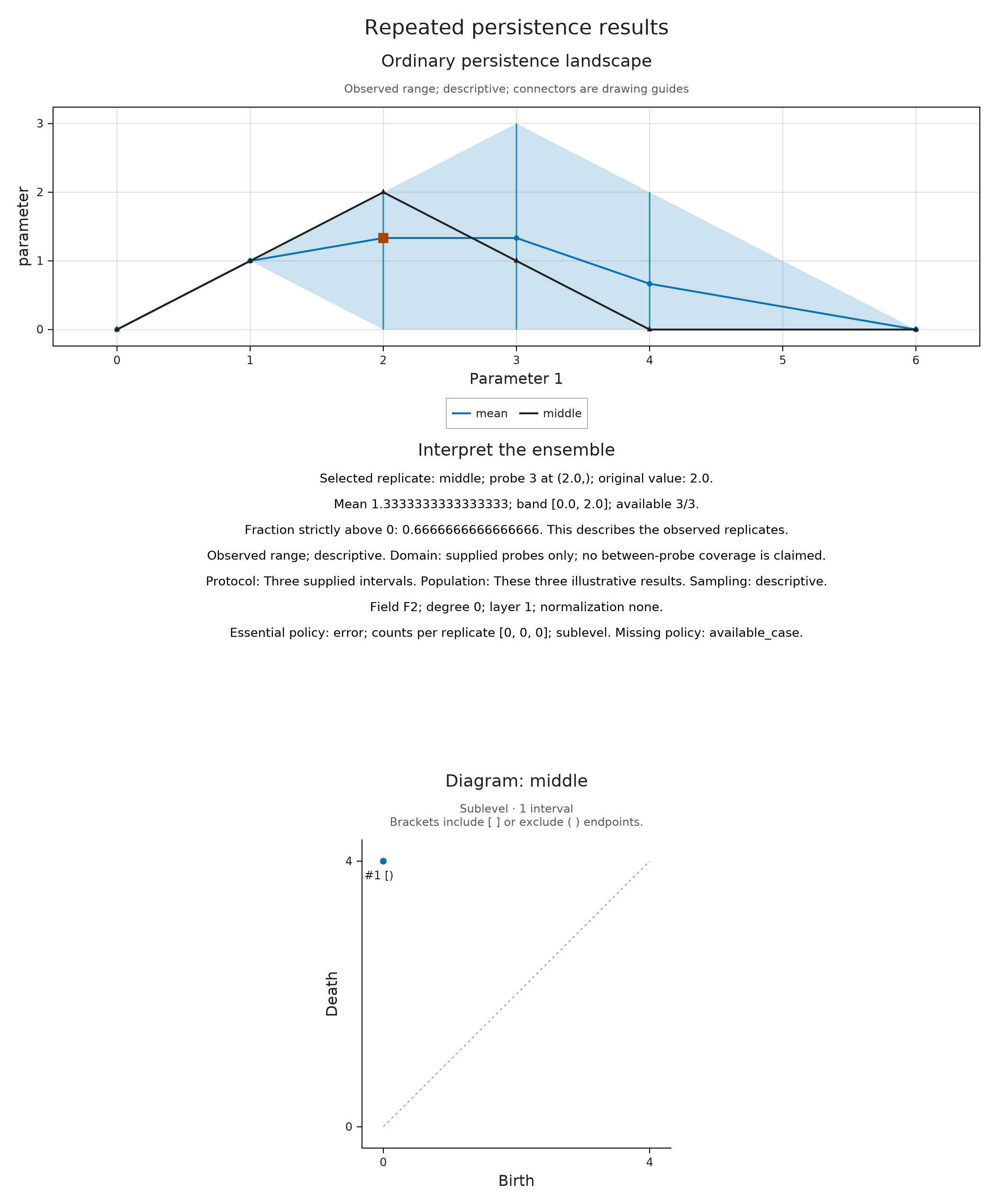
The markers are the probes at which we evaluated the tents. Segments and shading connect those sampled values so we can follow the picture; the summary itself contains no additional evaluations between them. In particular, a straight segment across a tent's corner need not reproduce that tent.
We can display the three supplied diagrams beside the summary to see where its variation comes from. This puts the observations in view without trying to identify a bar in one diagram with a bar in another.
In the prepared viewer, choose the short, middle and long intervals at $t=2$. Their selected heights are 0, 2 and 2, while the mean and observed range stay fixed. The final choice moves to the long interval at $t=3$: its height becomes 3, and the range at that probe is $[0,3]$, although the mean is still $4/3$. Every view uses the same three hand chosen rows; selection supplies no new observations or confidence claim.
OP.visualize(spread; diagram_samples=(1,2,3))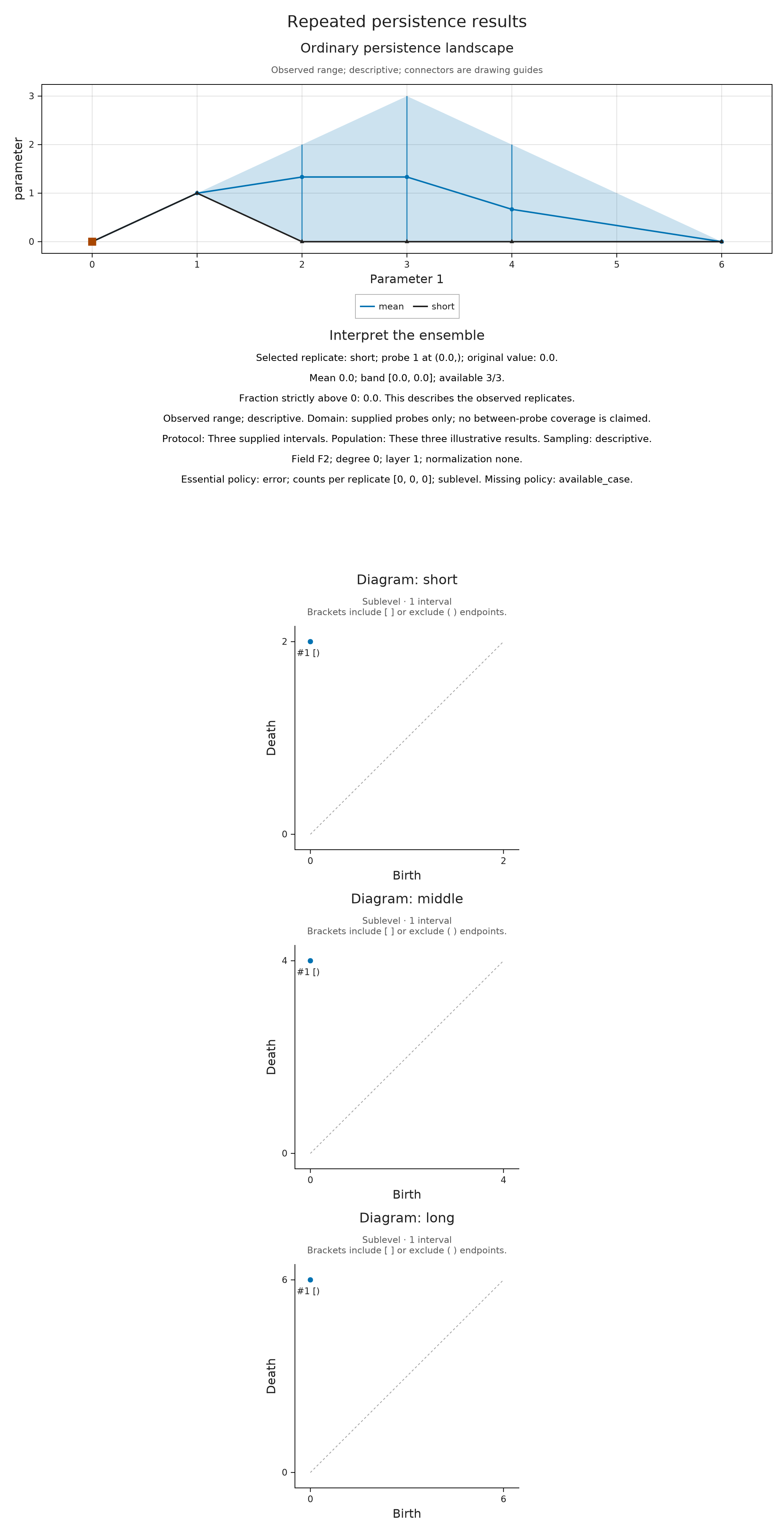
Read support frequencies
Instead of asking for an average height, we can ask how often the height exceeds a threshold. At $t=2$, two of the three rows are strictly positive, so the frequency above zero is $2/3$. In the following figure the vertical quantity is a fraction of the available observations, with values between zero and one. Its interpretation depends on the threshold and the rows we supplied; this descriptive calculation does not assign a confidence level to a population probability.
frequency = OP.summarize_ensemble(ensemble; threshold=0)
@assert OP.ensemble_values(frequency).frequency[3] == 2/3
OP.visualize(frequency; view=:frequency, probe=3)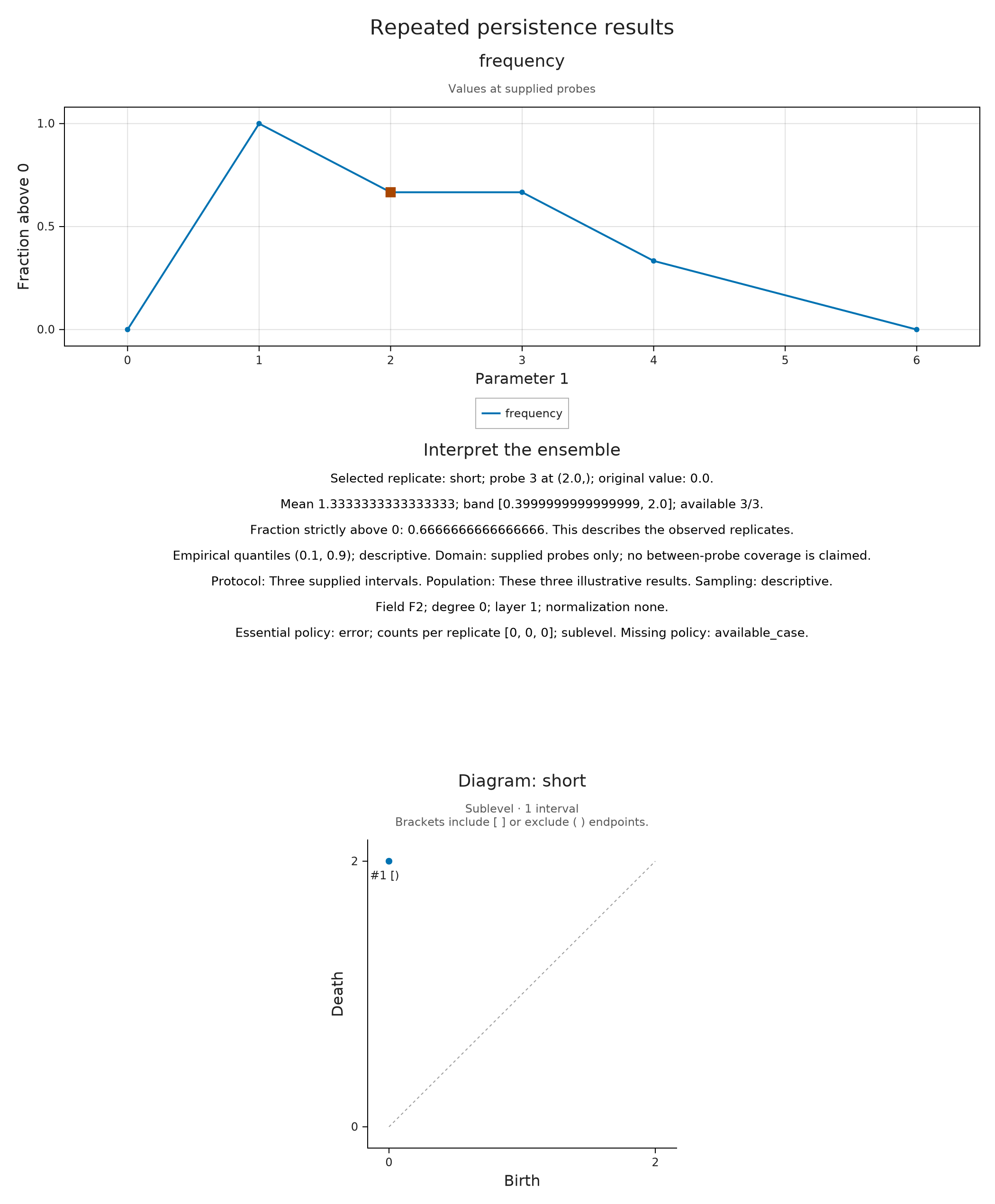
Try raising the threshold to 1 at $t=1$. The table shows three heights equal to 1, so none is strictly greater than the new threshold. We should therefore obtain frequency zero:
The two prepared views below make this comparison at the same marked probe $t=1$. The frequency axis remains fixed from 0 to 1 as the threshold changes, so the drop from all three rows to none is visible on the same scale.
above_one = OP.summarize_ensemble(ensemble; threshold=1)
@assert OP.ensemble_values(above_one).frequency[2] == 0
Compare finite modules at shared original parameters
A dimension query on a finite encoding gives another observable. Across several encodings, a column of our table should refer to the same original parameter, such as $(x,y)=(1,2)$. The finite label assigned to that point may differ between encodings, so matching vertex numbers alone would not establish that the queries agree.
For a small example, use a product of two two-element chains as the finite poset. Each of our two modules has just one nonzero stalk, the vector space at the least element. Its dimension is one in the first module and two in the second; every other stalk and every map along a covering relation is zero. Thus both paths around the square compose to zero. The following explicit construction uses the module owner APIs so that we can see those spaces and matrices. The coefficient field is $\mathbb Q$.
P = OP.FiniteFringe.ProductOfChainsPoset((2,2))
pi = OP.EncodingCore.GridEncodingMap(P,([0,3],[0,5]))
dims1, dims2 = [1,0,0,0], [2,0,0,0]
M1 = OP.Modules.PModule{OP.QQ}(P,dims1,Dict(e=>zeros(OP.QQ,dims1[e[2]],dims1[e[1]]) for e in OP.FiniteFringe.cover_edges(P));field=OP.CoreModules.QQField())
M2 = OP.Modules.PModule{OP.QQ}(P,dims2,Dict(e=>zeros(OP.QQ,dims2[e[2]],dims2[e[1]]) for e in OP.FiniteFringe.cover_edges(P));field=OP.CoreModules.QQField())
encoded = [OP.EncodingResult(P,M1,pi), OP.EncodingResult(P,M2,pi)]
2-element Vector{TamerOp.Results.EncodingResult{TamerOp.FiniteFringe.ProductOfChainsPoset{2}, TamerOp.Modules.PModule{Rational{BigInt}, TamerOp.CoreModules.CoeffFields.QQField, Matrix{Rational{BigInt}}, TamerOp.FiniteFringe.ProductOfChainsPoset{2}}, TamerOp.EncodingCore.GridEncodingMap{2, Int64, TamerOp.FiniteFringe.ProductOfChainsPoset{2}}, Nothing, Nothing, @NamedTuple{}}}:
EncodingResult(backend=auto, module_type=PModule, compiled=false, materialized=true)
EncodingResult(backend=auto, module_type=PModule, compiled=false, materialized=true)The encoding map assigns an original parameter pair to a finite label. We query the dimension of the vector space at that label and retain the original $(x,y)$ as the coordinates of the answer. ScalarField stores these sampled scalar values on their Cartesian grid; its plotted cells should be read as a view of the samples, not as a reconstruction of the encoding map's exact regions.
At the first probe, the two dimensions are 1 and 2. Their mean is $3/2$, and exactly one of them exceeds the chosen threshold 1. The frequency picture should show $1/2$ there and zero at probes where both modules vanish.
xgrid, ygrid = [0.,1.,3.,6.], [0.,2.,5.]
fields = [OP.ScalarField((xgrid,ygrid),
    [A.dim_at(OP.encoding_module(enc), A.locate(OP.encoding_map(enc),(x,y))) for x in xgrid, y in ygrid];
    id="module $i", units="dimension", axis_labels=("x","y")) for (i,enc) in enumerate(encoded)]
module_ensemble = OP.persistence_ensemble(fields; protocol="Two supplied finite modules",
    population="These algebraic examples", field="QQ")
module_spread = OP.summarize_ensemble(module_ensemble; threshold=1)
@assert OP.ensemble_values(module_spread).mean[1,1] == 1.5
@assert OP.ensemble_values(module_spread).frequency[1,1] == 0.5
OP.visualize(module_spread; view=:frequency)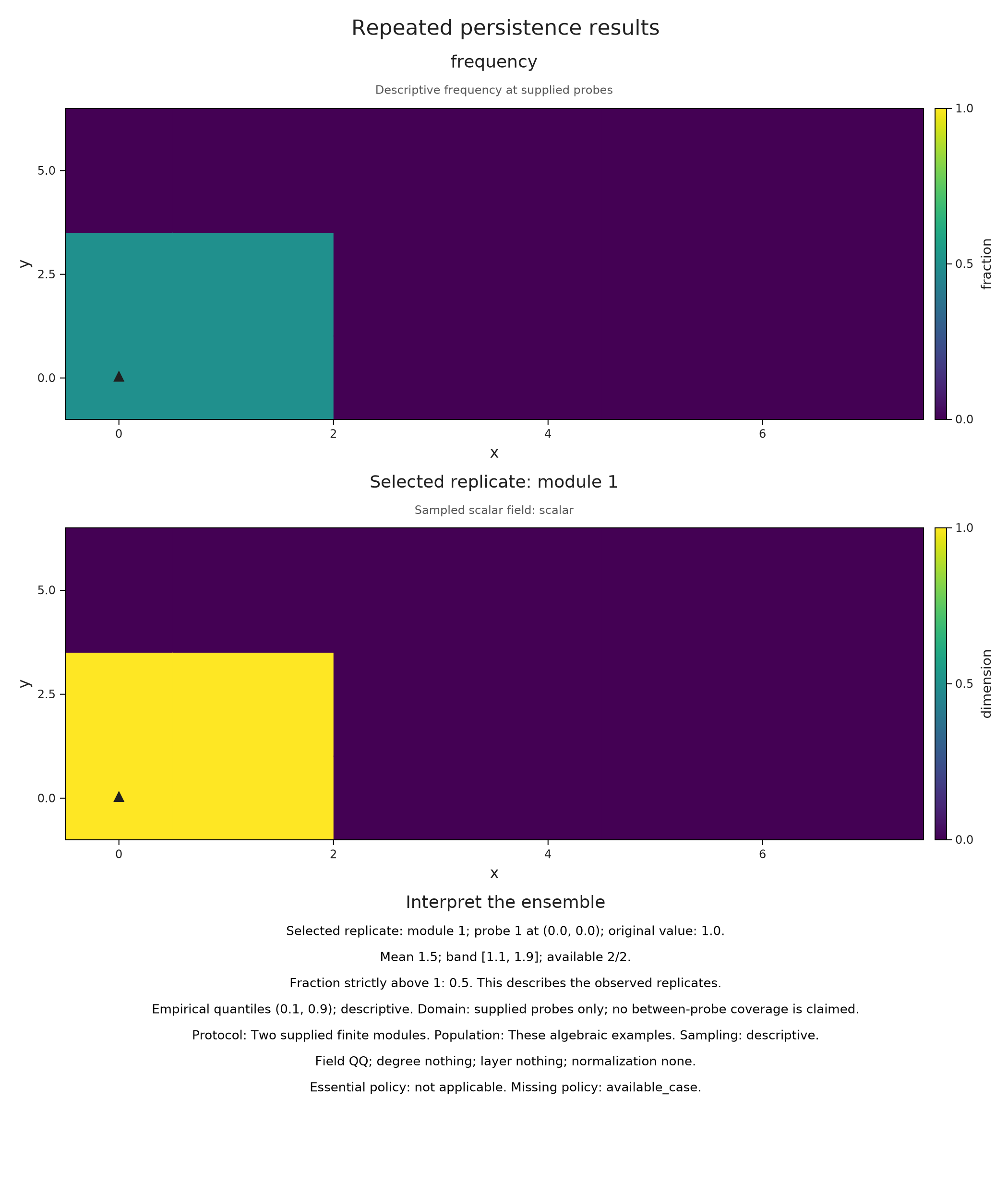
When a mean band supports inference
To infer a population mean, we need a sampling model. Assume that each row is an independent observation from the same distribution, that we fixed the probes before seeing the observations, and that the observable is known to lie in $[0,3]$. The assumption about the rows is called independent and identically distributed, abbreviated IID. Fixing the probes is a separate requirement. Independence concerns the rows: values at different probes within a row may depend strongly on one another.
The bound has to follow from the possible inputs. For example, if every interval is contained in $[0,6]$, each first landscape height is at most 3, regardless of which intervals we happen to observe. A sample's largest observed value would not justify the same claim about unseen intervals.
We reuse the three hand chosen rows below to illustrate the call and its resulting width. They do not become random observations when we set sampling=:iid. That option records the sampling assumption; an inferential use of this call requires independently sampled rows from the declared population. Repeated perturbations of one subject do not provide independent subjects.
iid_ensemble = OP.persistence_ensemble(diagrams; grid=[0.,1.,2.,3.,4.,6.],
    sample_ids=["short","middle","long"], sampling=:iid,
    protocol="Hand chosen rows illustrating an IID sampling assumption",
    population="A declared distribution of intervals with endpoints in [0,6]")
confidence = OP.summarize_ensemble(iid_ensemble; band=:hoeffding, bounds=(0,3), level=0.95)
OP.visualize(confidence; probe=3)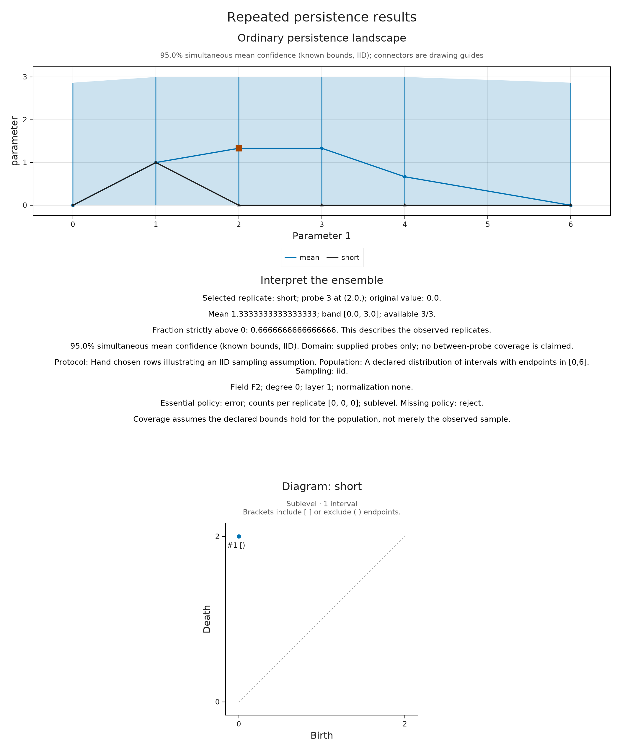
The mean band is wide because the formula has only three rows to work with. Under the stated sampling and boundedness assumptions, Hoeffding's inequality bounds the error at each probe. Adding the six error probabilities gives the simultaneous statement: repeated independent samples would produce intervals containing all six population means with probability at least 0.95. The implementation account derives the width.
With scope=:pointwise, the requested level applies separately to each probe. Simultaneous coverage asks for all the means to be inside their intervals at once, which is a stronger requirement and uses a larger radius before intersecting with the known bounds. After that intersection, some intervals can agree. Both statements concern the supplied probes and the chosen observable, so neither describes a confidence set for an entire persistence module.
A bootstrap offers an approximate approach when known population bounds are unavailable. It repeatedly draws whole rows with replacement from the observed table and compares their mean vectors with the original mean. Keeping a row intact preserves the relation between its probe values. This method still needs a suitable sampling model; a tiny, constant or dependent sample can give misleading widths. TamerOp retains the seed and number of resamples, but these choices do not confer a finite sample coverage guarantee.
bootstrap = OP.summarize_ensemble(iid_ensemble; band=:bootstrap,
    bootstrap_samples=500, seed=27, scope=:simultaneous)
@assert OP.ensemble_summary(bootstrap).contract.coverage == :approximate
OP.ensemble_summary(bootstrap)
(kind = :ensemble_summary, ensemble = (kind = :persistence_ensemble, samples = 3, probes = 6, shape = (6,), context = (statistic = "Ordinary persistence landscape", protocol = "Hand chosen rows illustrating an IID sampling assumption", population = "A declared distribution of intervals with endpoints in [0,6]", sampling = :iid, units = "parameter", axis_labels = ("Parameter 1",), degree = 0, field = "TamerOp.CoreModules.CoeffFields.PrimeField(2)", layer = 1, normalization = "none", essential = "error; counts per replicate [0, 0, 0]; sublevel"), missing = 0), contract = (band = :bootstrap, quantiles = (0.1, 0.9), threshold = 0, level = 0.95, scope = :simultaneous, coverage = :approximate, domain = :supplied_probes_only, bounds = nothing, bootstrap_samples = 500, seed = 27, missing_policy = :reject))Select a replicate and its source
Once the summaries are prepared, we can inspect individual observations alongside them. A supplied source figure is associated with its replicate ID, so selecting the second module brings its encoding picture into view. That association comes from the objects we supply; selection does not compute a new correspondence between them.
The next cell takes a static snapshot of this selection. The summary and its statistical assumptions stay the same when we change the selected replicate or probe.
sources = [(source=V.visual_spec(enc),) for enc in encoded]
session = OP.inspection_session(module_spread; samples=sources)
A.select_inspection!(session; sample="module 2", probe=1)
OP.visualize(A.inspection_snapshot(session))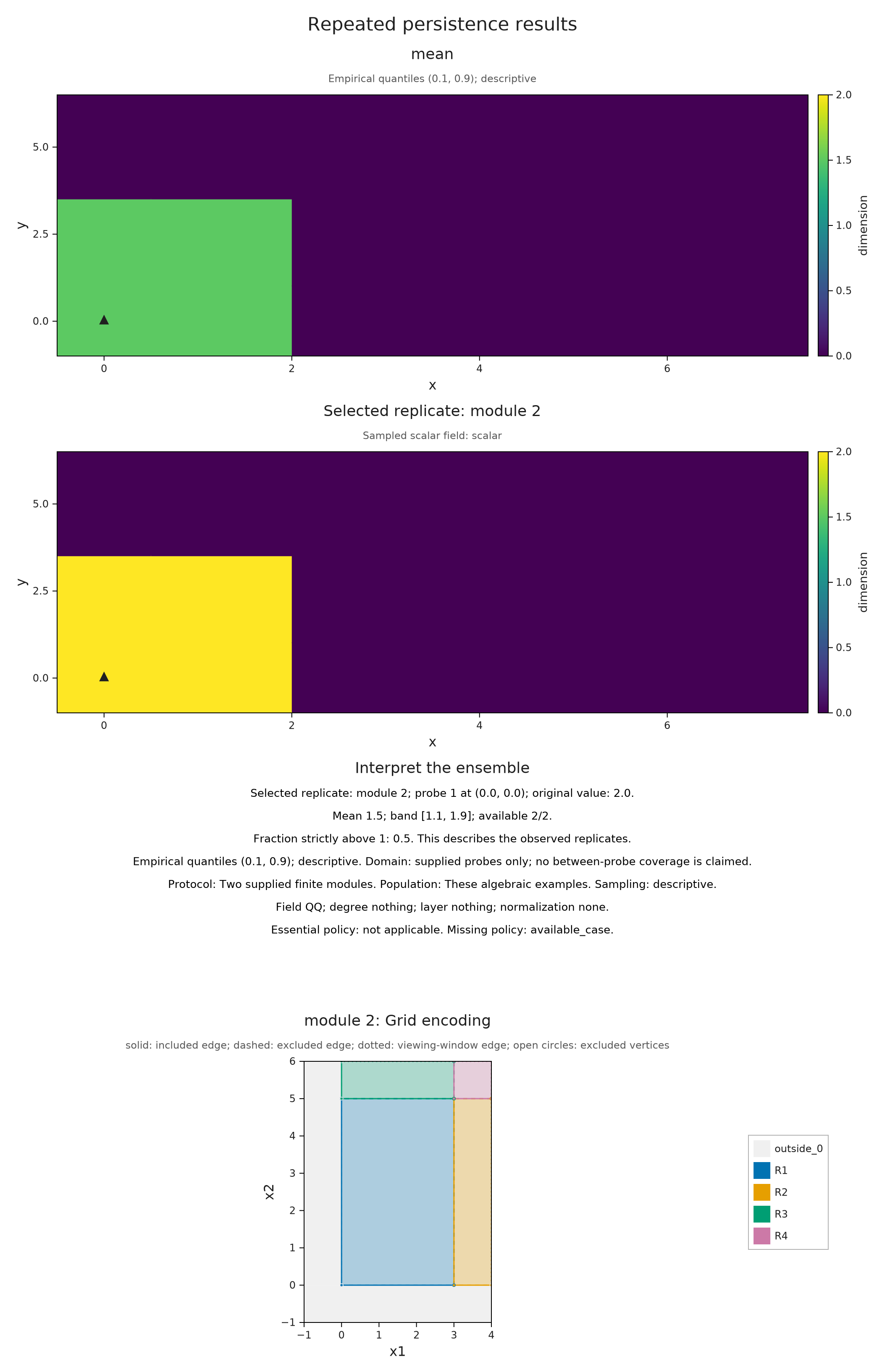
For a live view in a running Julia session, import WGLMakie and call OP.visualize(session; backend=:wglmakie). Pointer picking and the labelled replicate and probe inputs select the same prepared observations. Invalid input leaves the last valid selection visible. A static HTML scene retains a prepared picture; these controls require their Julia session, and notebook hosts have separate frontend requirements described in the display choices.
Release the session after inspection
Optional: release the session after inspection
A snapshot can still be displayed or exported after the session closes. Closing releases the session's input references and listeners. If you are finished with live selection, keep the snapshot and close the session here:
snapshot = A.inspection_snapshot(session)
A.close_inspection!(session)
@assert A.check_inspection_session(session).valid
Optional: save the prepared ensemble views
The browser examples select from figures prepared from the descriptive summaries above. Each saved choice retains its mathematical label, common plotting window and selected value. These exports do not resample the observations or turn the illustrative rows into a statistical sample.
replicate_choices = (
    (name="Short interval at t = 2", sample="short", row=1, probe=3, value=0.),
    (name="Middle interval at t = 2", sample="middle", row=2, probe=3, value=2.),
    (name="Long interval at t = 2", sample="long", row=3, probe=3, value=2.),
    (name="Long interval at t = 3", sample="long", row=3, probe=4, value=3.))
replicate_views = Pair{Symbol,Any}[]
for choice in replicate_choices
    prepared = OP.Advanced.visual_spec(spread; sample=choice.sample, probe=choice.probe)
    selected = prepared.metadata.selected
    @assert selected.value == choice.value
    @assert selected.mean ≈ 4/3
    @assert (selected.lower,selected.upper) == (0., choice.probe == 3 ? 2. : 3.)
    @assert prepared.panels[1].axes.ylimits == (-0.24,3.24)
    figure = OP.compose_visuals((
        heights=OP.visual_panel(prepared; panel=:ensemble_curve,
            context=OP.VisualContext(domain="Supplied parameter probes",
                units=("Parameter t", "Landscape height"),
                provenance="Three hand chosen intervals")),
        interval=OP.visual_panel(diagrams[choice.row]; kind=:barcode, dim=0,
            window=(0,6), title="Selected interval: $(choice.sample)"));
        columns=1, title="$(choice.name): height $(choice.value)",
        subtitle="Mean 4/3; observed range [$(selected.lower), $(selected.upper)] at this probe.")
    push!(replicate_views, Symbol(choice.name) => figure)
end
replicate_viewer_path = joinpath("tamerop_outputs", "ensembles", "replicates.html")
mkpath(dirname(replicate_viewer_path))
OP.save_visual_session(replicate_viewer_path,
    (; replicate_views...); selected=Symbol("Middle interval at t = 2"),
    title="Read a replicate beside the observed range",
    caption="These three hand chosen intervals are illustrative degree zero results over F₂. The blue curve is the mean; the black curve belongs to the selected interval. The orange square marks the mean at the selected probe. Shading describes their observed range at the supplied probes, with no population confidence claim. Lines between probes guide the eye; they add no evaluations.",
    style=OP.VisualStyle(fontsize=18), size=(760,850));
threshold_views = Pair{Symbol,Any}[]
for (threshold, summary, expected_count) in ((0,frequency,3), (1,above_one,0))
    prepared = OP.Advanced.visual_spec(summary; view=:frequency, probe=2)
    @assert prepared.metadata.selected.frequency == expected_count/3
    frequency_panel = OP.visual_panel(prepared; panel=:ensemble_curve,
        limits=(x=(0,6),y=(-0.05,1.05)))
    figure = OP.compose_visuals((frequency=frequency_panel,); columns=1,
        title="At t = 1: $expected_count of 3 heights exceed $threshold",
        subtitle="The selected probe has three heights equal to 1. Exceedance is strict.")
    push!(threshold_views, Symbol("Threshold $threshold at t = 1") => figure)
end
threshold_viewer_path = joinpath("tamerop_outputs", "ensembles", "thresholds.html")
mkpath(dirname(threshold_viewer_path))
OP.save_visual_session(threshold_viewer_path,
    (; threshold_views...); title="Change the threshold for the same observations",
    caption="The frequency is the fraction of the three supplied landscape heights strictly greater than the threshold at each probe. It describes these hand chosen intervals, without estimating a population probability. Both views use the same axes.",
    style=OP.VisualStyle(fontsize=18), size=(760,450));
The interval example makes the interpretation of a band depend on a question we can state explicitly: are we describing these observed heights, or using a sampling model to infer their population mean? The same distinction applies to dimensions and other observables of finite encodings once their query coordinates agree.
The API reference collects the input, missing-data and inference options; the implementation account follows the reductions and resampling. When the inputs are to be compared without a common sampling population, declared correspondences provides a different starting point.