Refining and transporting encoded modules
Download the executed notebook · Build and environment record
Two encodings can describe the same persistence module while dividing its parameter space differently. To compare them, we need to see how their labels correspond and how their linear maps act after that correspondence. This guide follows those data for a square, first through a common refinement and then through a change of finite base.
We assume the meaning of a space and structure map and a finite encoding. All coefficients below are rational, so matrix equations are exact. CairoMakie supplies the saved figures; the computations themselves use TamerOp. Along the way, we will see why identifying two modules after restriction is a more limited conclusion than identifying their derived categories.
The reference gives the complete input and return contracts. The implementation account explains how restrictions, limits and colimits are computed.
import TamerOp as OP
import CairoMakie
using LinearAlgebra: I

field = OP.CoreModules.QQField()
P = OP.Advanced.ProductOfChainsPoset((3, 3))
R = OP.Advanced.ProductOfChainsPoset((2, 2))
ProductOfChainsPoset
  axes: (2, 2)
  orientation: (1, 1)
  nvertices: 4
  model: finite product of chains
One square, two finite descriptions
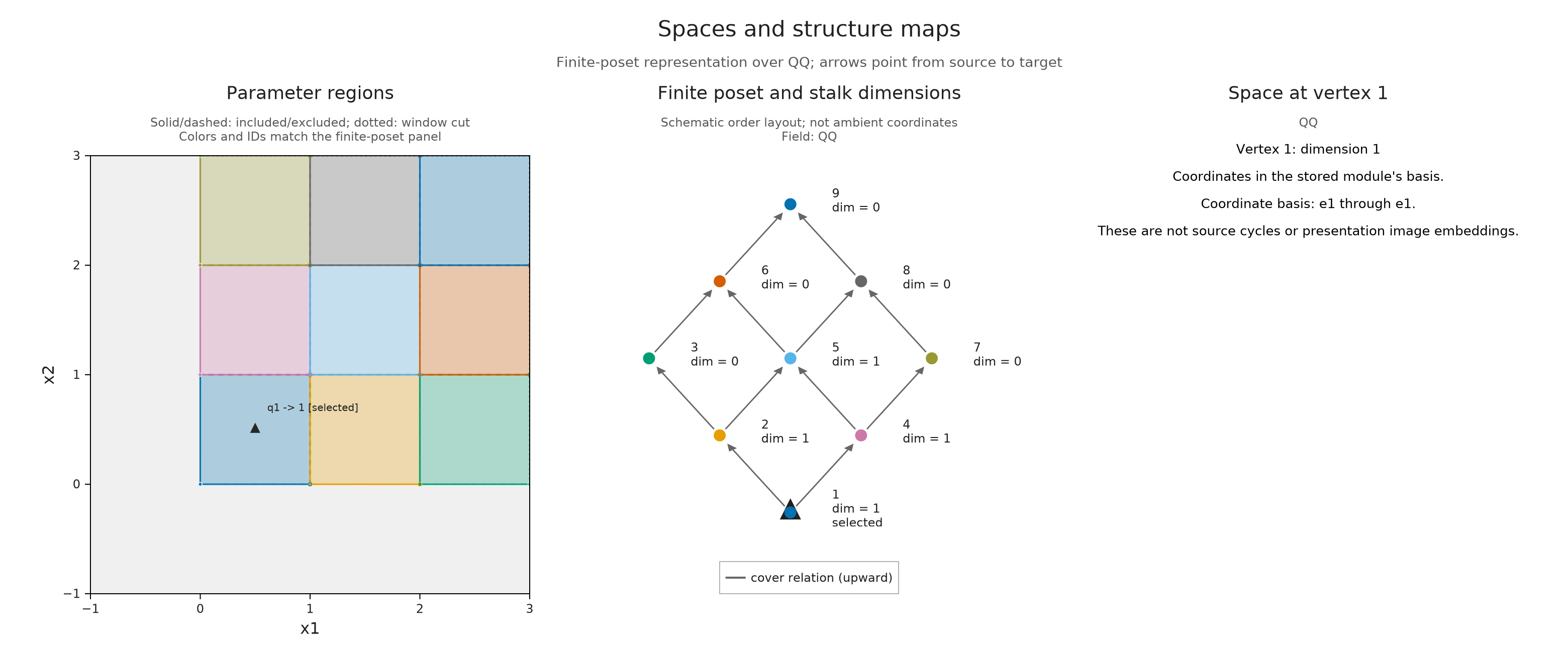
Work on the nonnegative parameter plane, with the coordinatewise order. Our module is one dimensional on $[0,2)\times[0,2)$ and zero elsewhere in that domain. The upper boundary is excluded, so the space at $(2,1)$ is zero. A negative coordinate lies outside the represented domain and has no supplied stalk. These conventions differ from the closed square used in the introductory encoding lesson.
The fine description divides each axis into $[0,1)$, $[1,2)$ and $[2,\infty)$; the coarse description uses $[0,2)$ and $[2,\infty)$. Their labels form product posets, ordered by increasing interval indices. In the code, the first coordinate varies fastest: the fine labels on the bottom row are 1, 2, 3, with 4, 5, 6 above them. Four fine labels therefore have a one dimensional space, while only one coarse label does.
We can construct these finite modules directly by supplying their dimensions and the matrices on cover relations, which are the order relations with no intermediate vertex. Inside the support each matrix is [1]. A map into a zero stalk has no rows, and a map out of one has no columns; ones with the corresponding dimensions constructs these empty matrices too.
left_dims = [1, 1, 0, 1, 1, 0, 0, 0, 0]
right_dims = [1, 0, 0, 0]
M = OP.Advanced.PModule{OP.QQ}(P, left_dims,
    Dict((a,b) => ones(OP.QQ, left_dims[b], left_dims[a]) for (a,b) in OP.Advanced.cover_edges(P)); field)
N = OP.Advanced.PModule{OP.QQ}(R, right_dims,
    Dict((a,b) => ones(OP.QQ, right_dims[b], right_dims[a]) for (a,b) in OP.Advanced.cover_edges(R)); field)
left = OP.EncodingResult(P, M, OP.Advanced.GridEncodingMap(P, ([0,1,2], [0,1,2])))
right = OP.EncodingResult(R, N, OP.Advanced.GridEncodingMap(R, ([0,2], [0,2])))
OP.visualize(left; kind=:module_inspector, point=(1//2,1//2), box=((-1,-1),(3,3)))
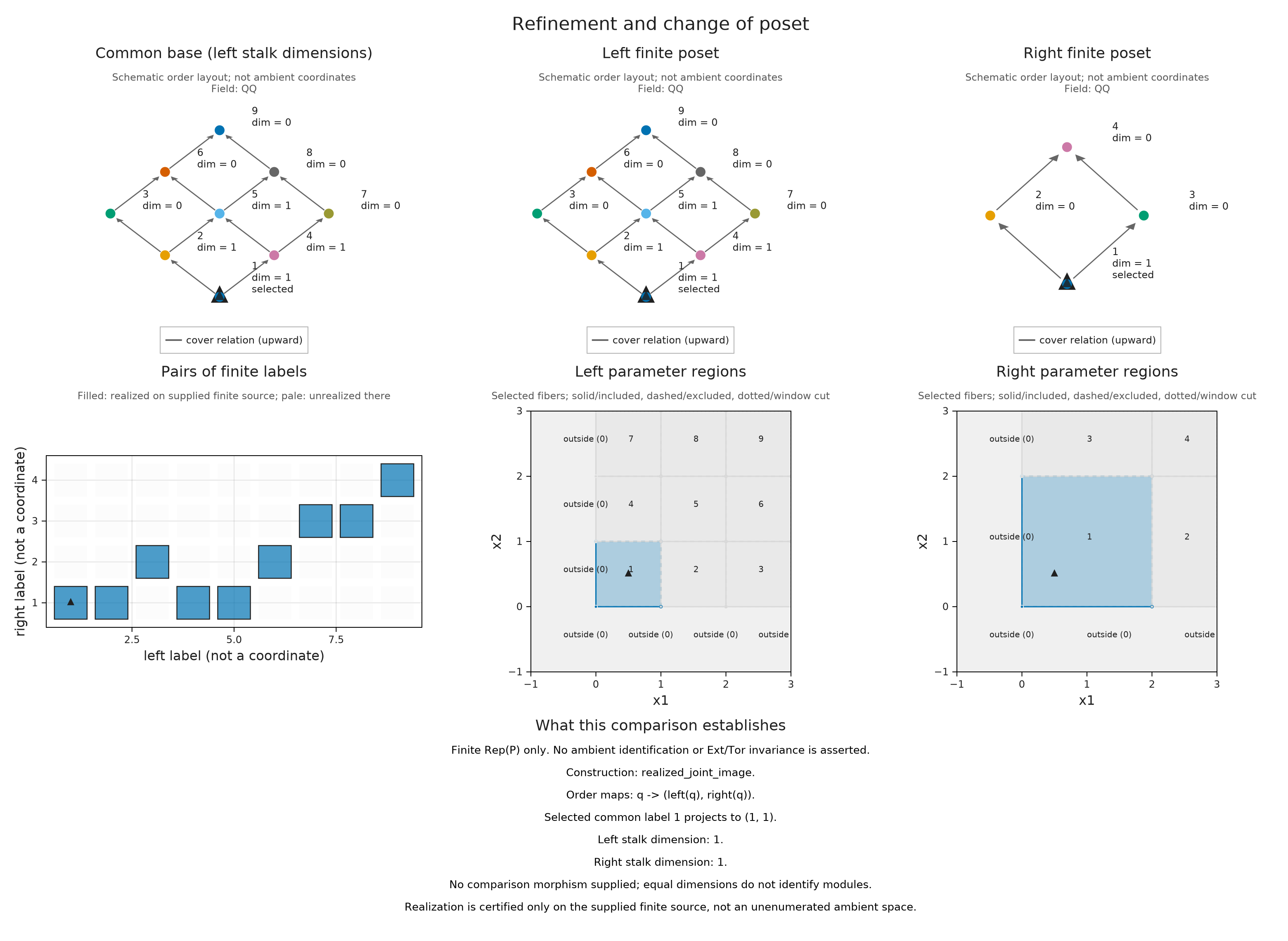
The two grid rules let us give an exact finite account of their overlap. Take the nine fine labels as a common source. The first map sends a label to itself, and the second sends it to the coarse rectangle containing its entire fiber. For example, labels 1, 2, 4 and 5 all go to coarse label 1.
joint_encoding collects the label pairs that actually occur on this source. A realized common base means this set of pairs with the order inherited from the product. There are nine pairs here, compared with the 36 pairs in the full Cartesian product. Restricting each module along the corresponding projection gives two modules on the same nine element poset.
The finite witness proves that these pairs occur on its declared nine labels. In this example, the grid formulas tell us more: every fine rectangle is nonempty and lies in the stated coarse rectangle, so the nine pairs describe the full nonnegative parameter plane. For arbitrary sampled parameters, that last conclusion would need a separate argument.
fine_classifier = OP.Advanced.EncodingMap(P, P, collect(1:9))
coarse_classifier = OP.Advanced.EncodingMap(P, R, [1,1,2,1,1,2,3,3,4])
joint = OP.Advanced.joint_encoding(fine_classifier, coarse_classifier)
refined = OP.common_refinement(left, right, joint)
OP.visualize(refined; sources=(left,right), joint, point=(1//2,1//2), box=((-1,-1),(3,3)))
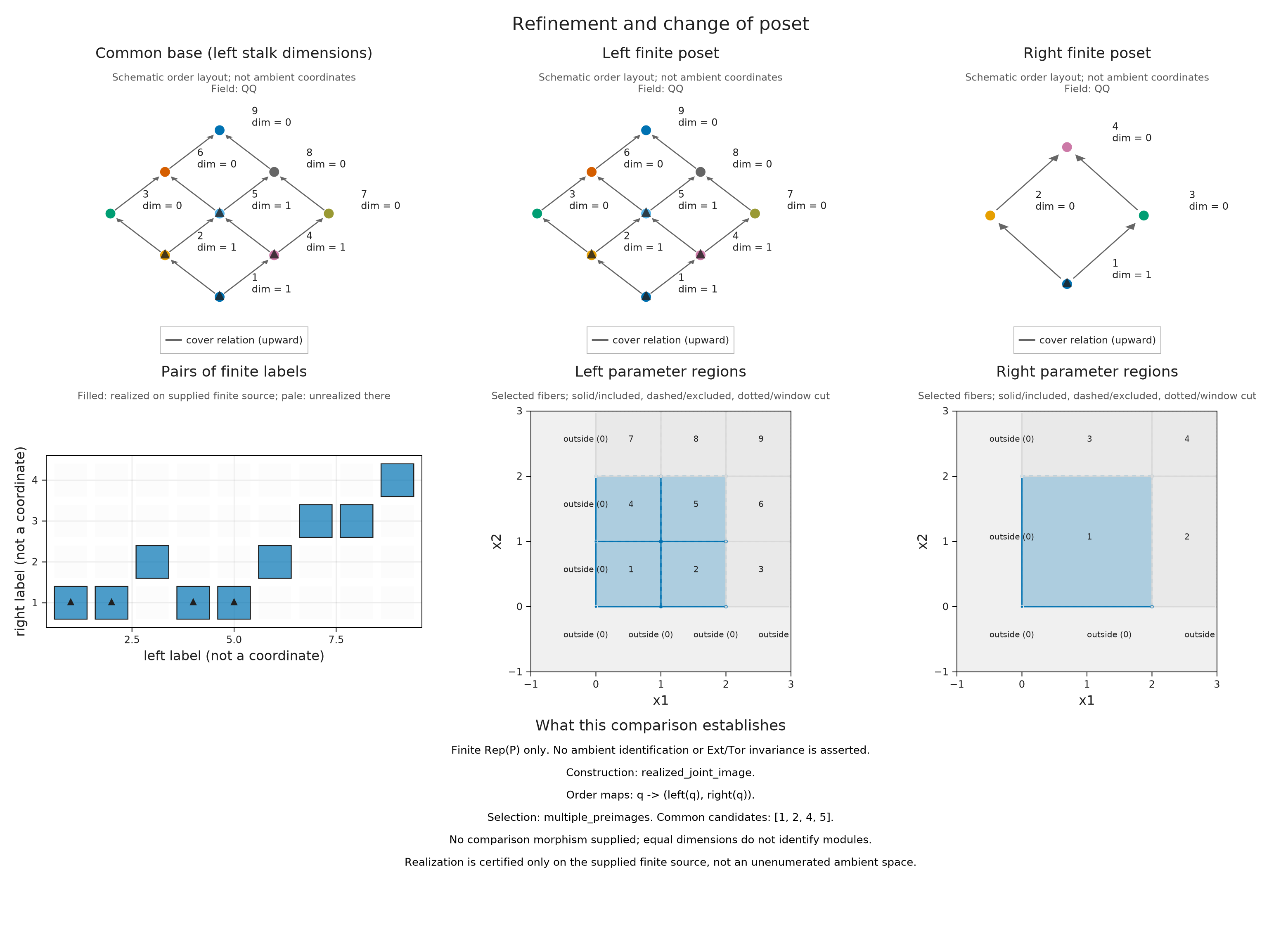
Select coarse label 1 to see its four preimages. They are distinct regions in the fine description even though the coarse module uses the same space and coordinates on all of them. The view keeps all four visible, which is useful when a comparison cannot be read from one chosen representative.
OP.visualize(refined; sources=(left,right), joint, side=:right, label=1, box=((-1,-1),(3,3)))
Supply the identification, then check its squares
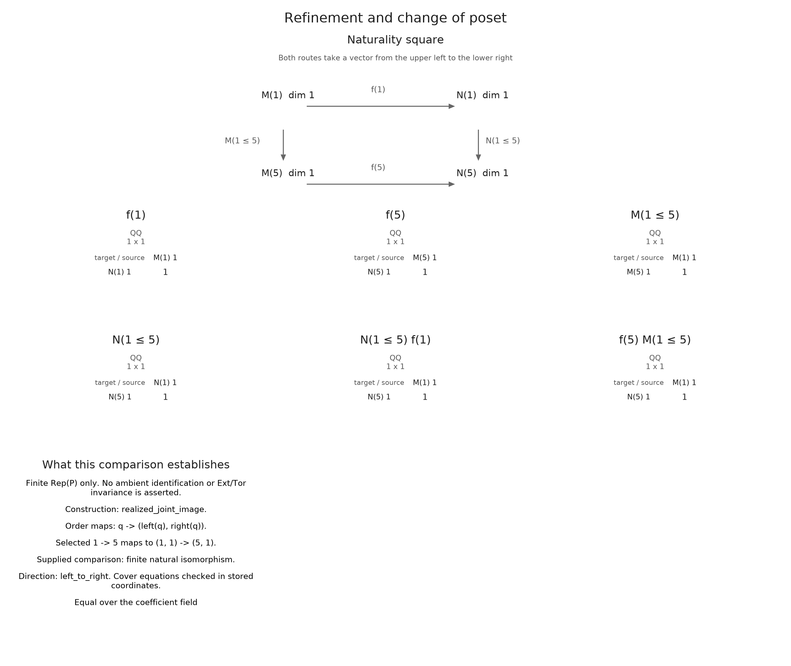
Write $L$ and $R$ for the two modules on the common base. A natural identification consists of invertible component maps $f_q:L(q)\to R(q)$ that commute with structure maps. For each $q\leq q'$, this asks for
\[R(q\leq q')f_q=f_{q'}L(q\leq q').\]
Both sides follow a vector from $L(q)$ to $R(q')$: one changes coordinates first and the other moves through the module first. Because our two descriptions used the same coordinates, we can supply identity components, including the empty identity at a zero stalk. Equal dimensions alone would not justify this choice for other modules.
translated_modules returns the actual restrictions as left and right. The figure checks the component ranks and all cover squares, then displays the four matrices and both composites for the selected pair. Covers suffice because each input module already has compatible composites along its order.
modules = OP.Advanced.translated_modules(refined)
comparison = OP.Advanced.PMorphism(modules.left, modules.right,
    [Matrix{OP.QQ}(I,d,d) for d in OP.dimensions(modules.left).stalks])
OP.visualize(refined; comparison, pair=(1,5), view=:square)
Zero targets and incomparable labels
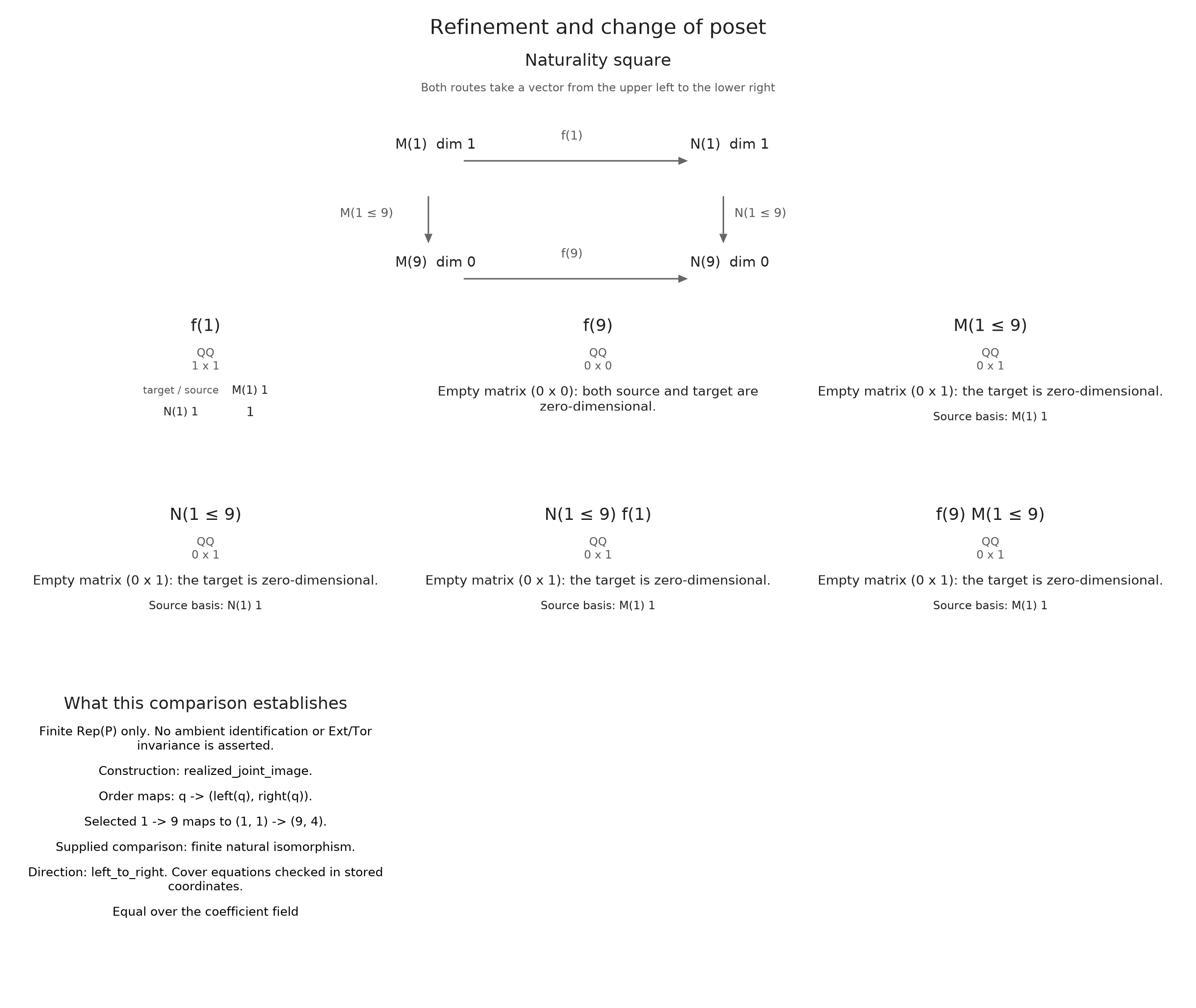
The fine label 9 represents parameters with both coordinates at least 2. Its stalk is zero, so the map from label 1 to label 9 is the unique map from $\mathbb{Q}$ to zero. The selected square still commutes: both paths have a 0 × 1 matrix.
OP.visualize(refined; comparison, pair=(1,9), view=:square)
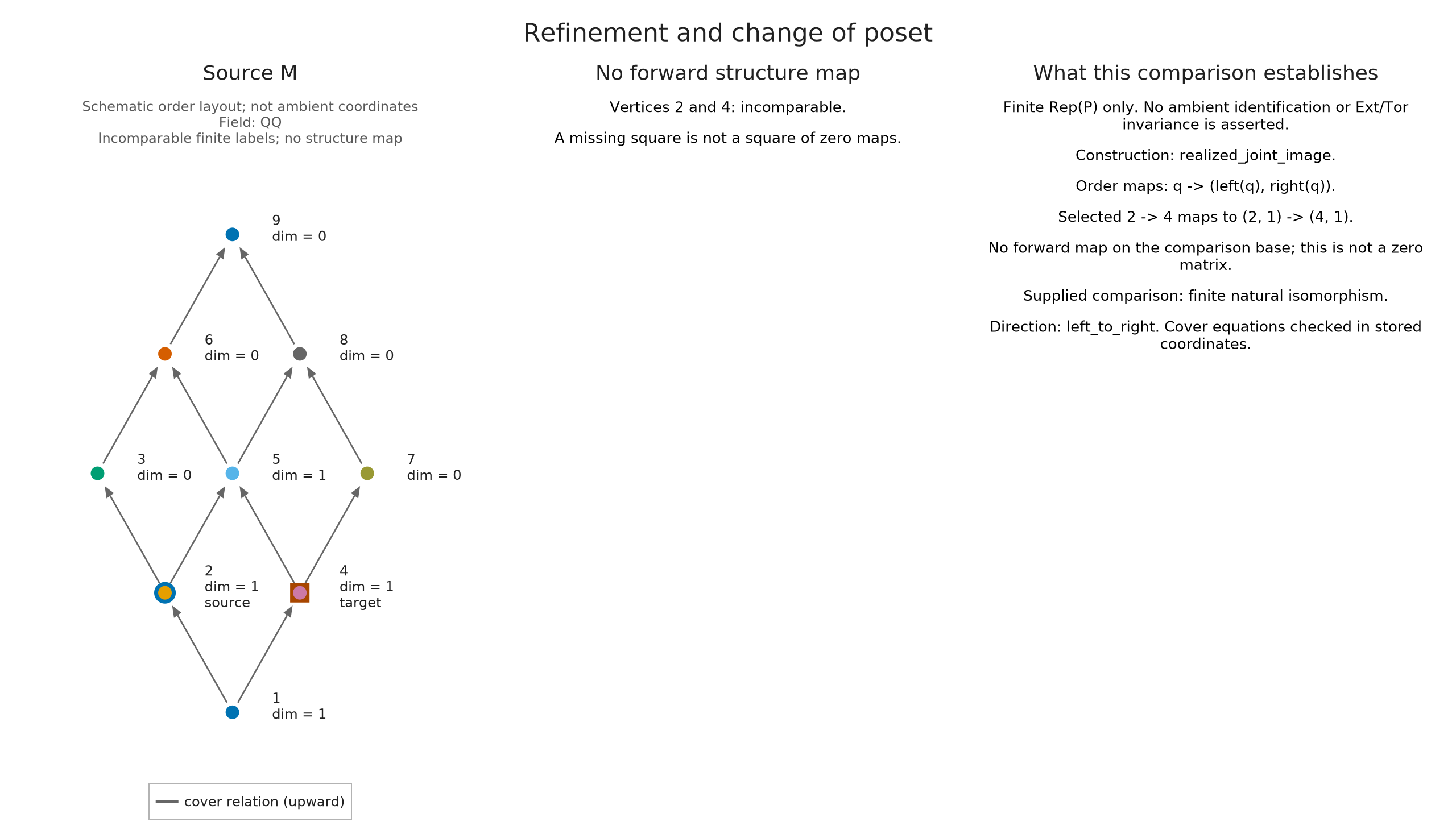
OP.visualize(refined; comparison, pair=(2,4), view=:square)
Compare the three pairs
Choose a pair to follow the identification around its square. From 1 to 5 both composites are identities; from 1 to 9 both have zero rows and one column. The pair 2 and 4 has no forward square. The two product matrices let us compare the routes without treating an absent map as a zero map.
Compare the naturality squares
The pair (2,4) uses labels 2 and 4, corresponding to rectangles on opposite sides of the lower left rectangle. Neither label is below the other, so there is no forward structure map and no naturality square for that pair. This absence has a different meaning from the defined zero map into label 9.
Restrict along the coarse classifier
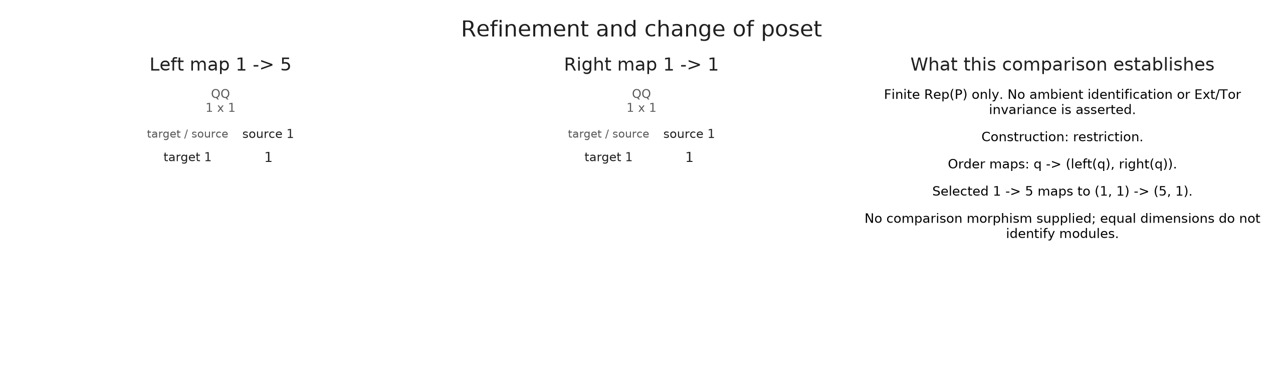
The same comparison can be approached by restricting the coarse module directly. If $\pi:P\to R$ is the coarse classifier, its restriction has space $N(\pi(p))$ at fine label $p$, and uses the map of $N$ between the projected endpoints. The order map runs from the new base to the old one, while restriction brings the module back to the new base.
The returned translation keeps the original encoding and the order map. In general, those data do not determine an ambient classifier into the new base, so the operation does not invent one. Here we already have the fine grid separately.
restricted = OP.restriction(coarse_classifier, right)
OP.visualize(restricted; pair=(1,5), view=:square)
Optional: compare with the entire product
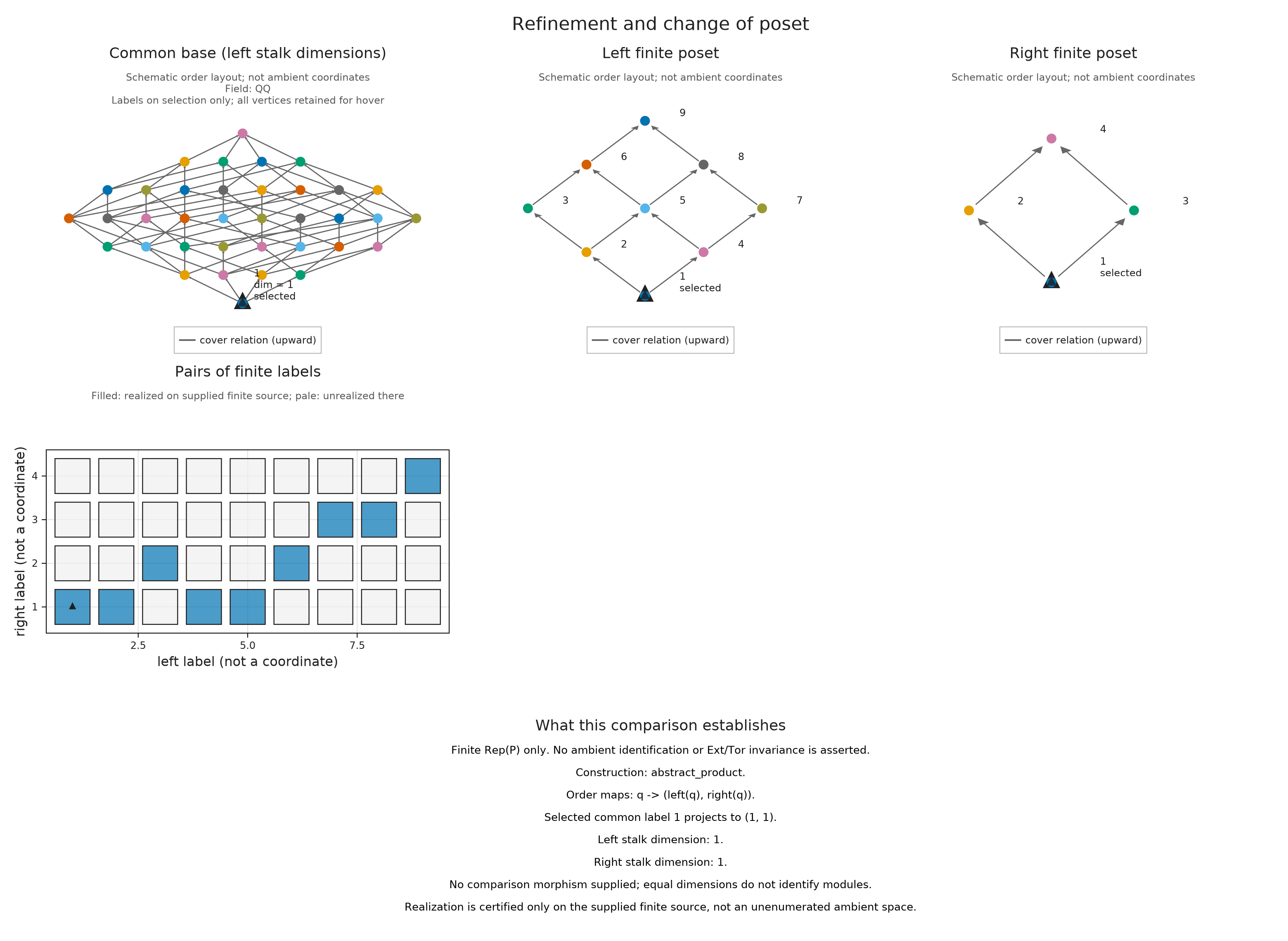
If we omit the joint witness, common_refinement uses an abstract product when the two finite bases differ. Every pair of labels then belongs to the common base, even if no original parameter receives that pair of labels. Passing joint to the viewer marks the nine pairs that occur on our finite source; it leaves the product module and its other labels in place.
product = OP.common_refinement(left, right)
OP.visualize(product; joint, vertex=1)
A Kan comparison does not identify finite derived categories
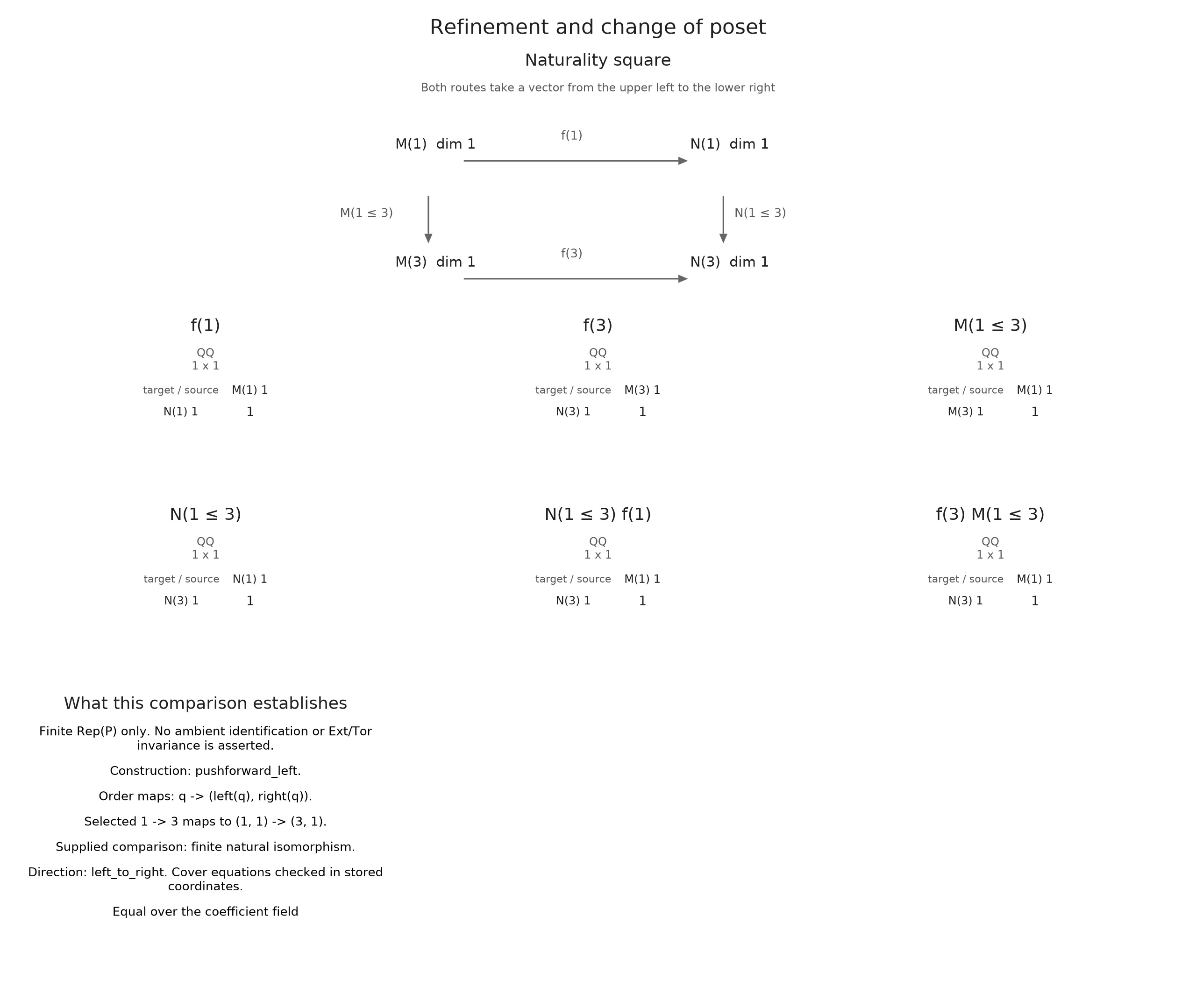
Restriction reads an existing module at the labels supplied by an order map. To go in the other direction, a left Kan extension combines the source spaces by identifying vectors with their images along the source maps. At a target label $p$, it uses the source labels $q$ whose images satisfy $\pi(q)\leq p$. This combination is a colimit: maps out of it correspond to compatible maps out of those source spaces.
Consider an order map that collapses a connected finite poset $Q$ to one point. Let $C$ be the constant module with space $\mathbb{Q}$ and identity maps. The colimit identifies all these copies of $\mathbb{Q}$, so the left Kan extension is one copy of $\mathbb{Q}$. Its pullback is again constant on $Q$. The canonical map from $C$ to that pullback is called the left Kan unit, and each of its components is invertible in this example.
Take $Q$ to have two minimal and two maximal elements, with each minimum below each maximum. Its order complex, formed by making a simplex for each nonempty chain, is a cycle with four edges. The degree one self-Ext of $C$ has dimension one, while the self-Ext of a vector space at one point is zero in positive degrees. Here Ext measures classes of extensions in the specified representation category; the category lesson derives this example and explains the hypotheses needed for derived comparisons.
We first compute the left Kan extension and its unit, then inspect the unit on a selected pair. The finite bases remain explicit throughout the calculation.
Q = OP.Advanced.FinitePoset(Bool[1 0 1 1; 0 1 1 1; 0 0 1 0; 0 0 0 1])
point_poset = OP.Advanced.FinitePoset(trues(1,1))
C = OP.Advanced.PModule{OP.QQ}(Q, ones(Int,4),
    Dict(edge => ones(OP.QQ,1,1) for edge in OP.Advanced.cover_edges(Q)); field)
collapse = OP.Advanced.EncodingMap(Q, point_poset, ones(Int,4))
encoded_C = OP.EncodingResult(Q,C,nothing)
transported = OP.pushforward_left(collapse, encoded_C)
unit = OP.Advanced.kan_unit(collapse,C)
OP.visualize(transported; comparison=unit, pair=(1,3), view=:square)
options = OP.Advanced.DerivedFunctorOptions(maxdeg=1, model=:projective)
V = OP.translated_module(transported)
self_ext_Q = OP.Advanced.Ext(C,C,options)
self_ext_point = OP.Advanced.Ext(V,V,options)
@assert OP.Advanced.dim(self_ext_Q,1) == 1
@assert OP.Advanced.dim(self_ext_point,1) == 0
(ext1_on_Q=OP.Advanced.dim(self_ext_Q,1), ext1_on_point=OP.Advanced.dim(self_ext_point,1))
(ext1_on_Q = 1, ext1_on_point = 0)Optional: take the right Kan extension
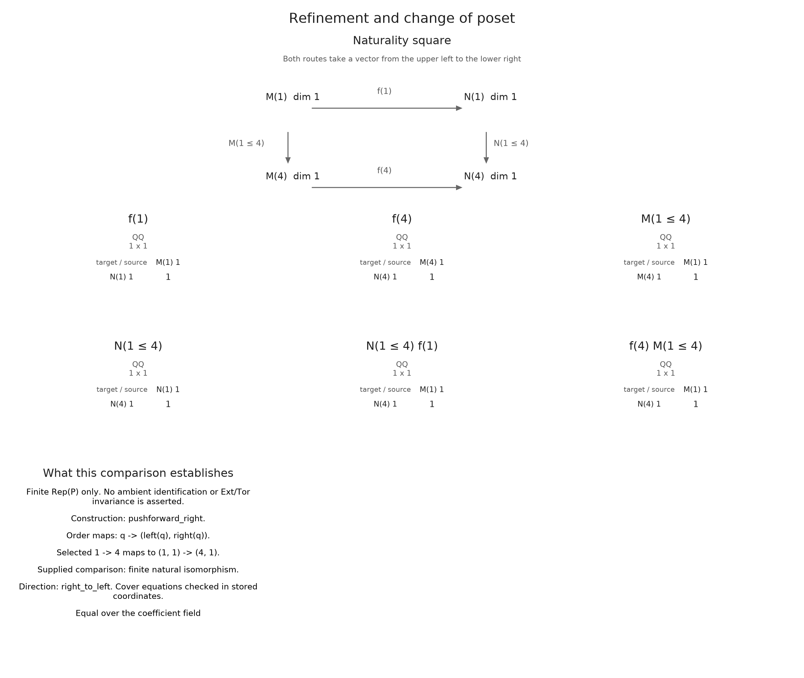
A right Kan extension uses a limit instead: at a target label $p$, its vectors are compatible families in the source spaces with $p\leq\pi(q)$. For our collapse to one point, an element of the limit assigns the same scalar to every vertex of the connected poset. The limit is therefore one dimensional too.
Projection from a compatible family to each of its entries gives the right Kan counit, from the pulled back limit to $C$. Its direction is opposite to the unit we just inspected, so we declare direction=:right_to_left. The viewer uses the Kan extension and comparison we supply; these algebraic constructions are separate calls.
right_transport = OP.pushforward_right(collapse, encoded_C)
counit = OP.Advanced.kan_counit(collapse,C; side=:right)
OP.visualize(right_transport; comparison=counit, direction=:right_to_left, pair=(1,4), view=:square)
Explore and test a prediction
The common refinement lets us move between the two square descriptions without losing either label. We can try the change from $(1/2,1/2)$ to $(3/2,3/2)$: the fine label should change from 1 to 5, while the coarse label remains 1. Both stalks are still one dimensional.
An inspection session retains the prepared comparison and lets us select several answers in succession. The following cell first checks the four preimages of coarse label 1, then selects the new parameter and draws a static snapshot. It needs no live browser connection.
session = OP.inspection_session(refined; sources=(left,right), joint, comparison, box=((-1,-1),(3,3)))
OP.Advanced.select_inspection!(session; side=:right, label=1)
@assert OP.Advanced.inspection_summary(session).candidates == [1,2,4,5]
OP.Advanced.select_inspection!(session; point=(3//2,3//2))
@assert OP.Advanced.inspection_snapshot(session).metadata.selection.query_labels == (5,1)
OP.visualize(OP.Advanced.inspection_snapshot(session))
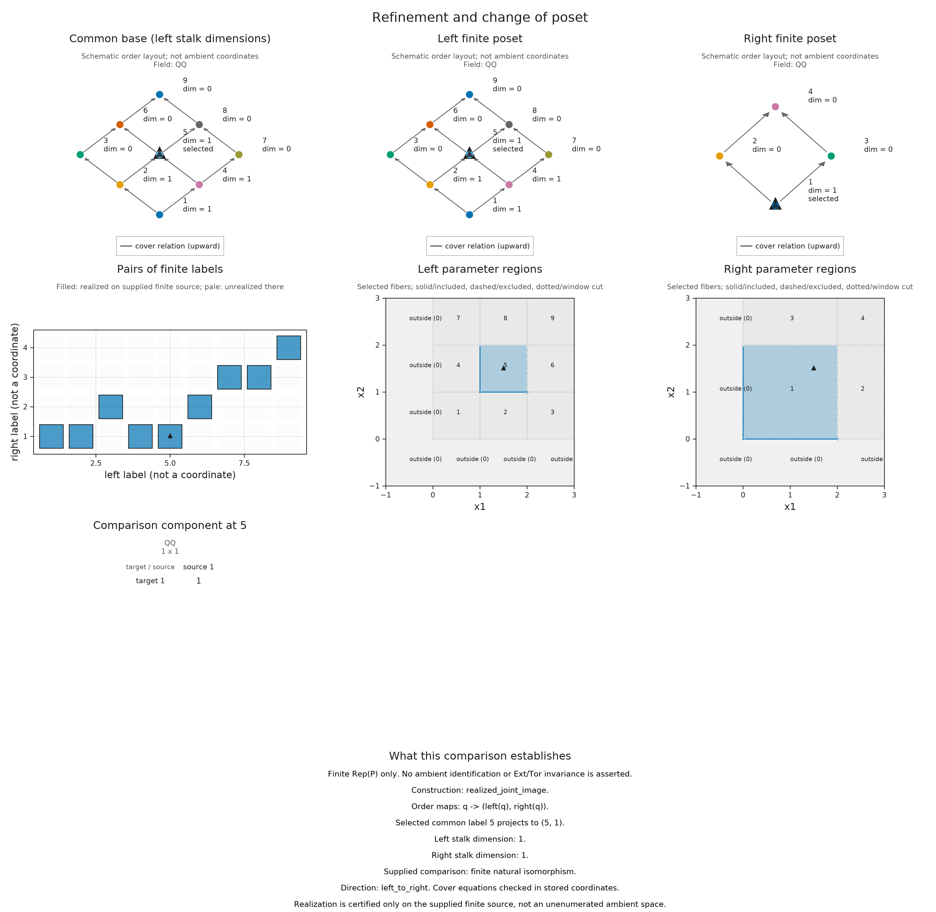
The snapshot shows the same parameter classified by both grids. Its coordinates, the two finite labels and the common label are related by the maps we supplied; the Hasse layout only draws their order.
Preparation validates modules and cover maps, and materializes any supplied lazy encodings. Keep the inputs unchanged while the session is open. close_inspection! releases its retained inputs and listeners while preserving the final static snapshot.
OP.Advanced.close_inspection!(session)
@assert OP.Advanced.check_inspection_session(session).valid
Optional: prepare the comparison views
Each view uses the same comparison morphism. We keep its square and the two computed composites, or the order diagram when no square exists. The files store these prepared choices for the browser.
square_labels = ["Inside: 1 to 5", "Into zero: 1 to 9", "Incomparable: 2 and 4"]
square_pairs = [(1,5), (1,9), (2,4)]
square_views = []
for (label, pair) in zip(square_labels, square_pairs)
    answer = OP.Advanced.visual_spec(refined; comparison, pair, view=:square)
    equation = answer.metadata.naturality
    if equation.defined
        @assert equation.valid && equation.left == equation.right
        @assert size(equation.left) == (pair == (1,5) ? (1,1) : (0,1))
        drawing = OP.compose_visuals((
            square=OP.visual_panel(answer; panel=1),
            first_route=OP.visual_panel(answer; panel=6),
            second_route=OP.visual_panel(answer; panel=7));
            columns=3, title=label, subtitle="Both routes use the supplied comparison over Q.")
    else
        @assert equation.relation == :incomparable
        drawing = OP.compose_visuals((
            order=OP.visual_panel(answer; panel=1),
            relation=OP.visual_panel(answer; panel=2));
            columns=2, title=label)
    end
    push!(square_views, drawing)
end
prepared_squares = NamedTuple{Tuple(Symbol.(square_labels))}(Tuple(square_views))
comparison_directory = joinpath("tamerop_outputs", "comparison")
mkpath(comparison_directory)
OP.save_visual_session(joinpath(comparison_directory, "squares.html"), prepared_squares;
    selected=Symbol(first(square_labels)), size=(1560,650),
    title="Compare the two routes through a square",
    caption="The two restrictions use rational coefficients and identity comparison components. Comparable pairs have equal composites; incomparable labels have no square.");
The square comparison used an explicit natural identification on a declared common base. This is the information needed to follow a vector consistently through the two descriptions. Changing one nonzero component of comparison to zero would make an adjacent cover square fail even though the dimensions stayed the same; changing coordinate bases instead would require the corresponding invertible component matrices.
For computations that depend on the finite category, continue with resolutions. The Kan example shows why it matters to record that category alongside the module.
Optional: inspect the comparison with a live Julia session
In a Julia environment with WGLMakie installed, create a new session after closing the one above. Copy this Julia example into a notebook code cell:
import WGLMakie
live_session = OP.inspection_session(refined;
    sources=(left,right), joint, comparison, box=((-1,-1),(3,3)))
OP.visualize(live_session; backend=:wglmakie)
The controls accept labels, exact parameter coordinates and directed pairs on the common base. A click on a Hasse vertex selects all its preimages; hovering reads retained labels without asking for new algebra. Multiple viewers can share the session. Closing one viewer releases its own callbacks; call OP.Advanced.close_inspection!(live_session) when you have finished with the session itself. The prepared comparison above switches among the three computed pairs; this live session can answer a new selection.
The reference describes the display limits: max_vertices=200 bounds the finite poset drawn, max_pairs=2500 bounds an optional Cartesian background, and matrix_limit=(12,12) crops displayed entries while retaining the full matrices and comparison equations.