Axis-aligned box encoding
Suppose a module is nonzero only on a line or at a single point. Sampling the open regions of a grid can miss its entire support. To encode it, the grid must retain the closed boundaries as cells in their own right, with their vector spaces and the maps entering and leaving them. This account follows how the box encoder makes those boundary cells part of a finite poset.
The indicator presentation lesson explains why a matrix between upset and downset indicators describes a module; the finite encoding introduction explains recovery through the map assigning each parameter its finite label.
The finite encoding viewpoint comes from Ezra Miller's theory of modules over posets, discussed in that introduction. The event grid below is the package's specialized construction for indicator presentations whose boundaries are parallel to coordinate axes.
A closed point needs three cells
Work over the rational field. Consider one parameter, the upset $U=[0,\infty)$, the downset $D=(-\infty,0]$, and the $1\times1$ coefficient matrix $[1]$. At a parameter $x$, the represented vector space is the image of the active matrix block. That space is one dimensional only at $x=0$.
The classifier assigns a finite label by recording two values: $y=1$ when $x\in U$, and $z=1$ when $x\notin D$, with zero in the respective other cases. Together, $(y,z)$ is the cell's signature. Using the complement of the downset makes both entries increase with the parameter:
| Parameter cell | $(y,z)$ | Fiber dimension |
|---|---|---|
| $x<0$ | $(0,0)$ | $0$ |
| $x=0$ | $(1,0)$ | $1$ |
| $x>0$ | $(1,1)$ | $0$ |
Crossing zero therefore has two events. At zero the upset becomes active; immediately after zero the downset ceases to be active. Keeping the intermediate state retains the point module. Merging these events would lose it.
Internally, the sorted axis wall sequence is [0.0, 0.0]. The cell between equal walls is their singleton. At a wall carrying only a birth, equality belongs to the cell on the right; at a wall carrying only a death it belongs to the cell on the left. Those walls need only one event because the boundary has the neighboring cell's signature. Repeating a wall in the stored sequence adds cells precisely where the closed birth and death conditions require them.
Products of these axis cells retain faces and corners. For example, $U=[0,\infty)^2$ and $D=(-\infty,0]\times(-\infty,2]$ with coefficient $[1]$ give a module supported on the segment $\{0\}\times[0,2]$. Along the segment the nonzero structure maps are identities; maps entering from or leaving to a zero space are zero. Ambient area alone cannot recover that information.
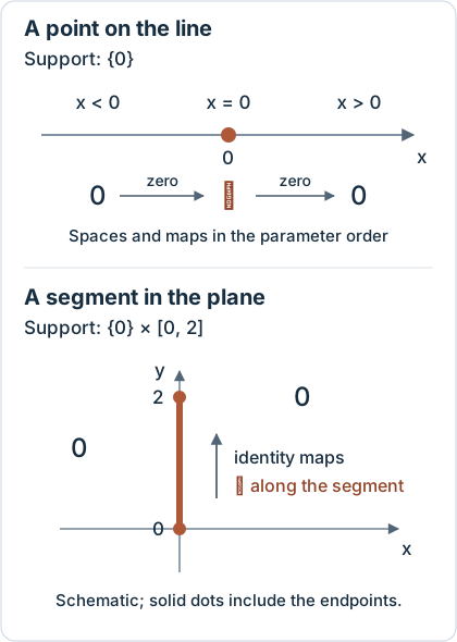
The marked endpoints belong to the support. The upper example needs a separate singleton cell; the lower one needs that cell along one axis and an interval along the other. Zero length or area in the ambient space does not imply a zero vector space.
Compare points on the segment with its neighboring open regions. The classifier has to distinguish them even though a drawing gives the segment no area. The choices below also include both closed endpoints.
- Signature (y, z)
- (1, 0)
- Represented vector space
- Q (dimension 1)
The solid blue segment is the support. The outlined orange circle marks the query. Here y records membership in the upset and z records being outside the downset, as above.
Traverse events, then identify equal signatures
The encoder visits the cell product with its first axis varying fastest. For each generator it maintains the number of satisfied coordinate inequalities. Moving through one axis event updates only generators with that threshold. The reverse updates restore the state when the traversal carries to the next axis. The maintained counts therefore let the encoder update a signature without testing every generator against each new cell.
The current zero and one entries of $(y,z)$ are packed into machine words and used as a dictionary key. Equal signatures share a region label, and the cell table retains the label for each visited cell. The finite order is componentwise inclusion of the two bit families. The resulting fringe presentation carries the original coefficients wherever its indicator intersection is nonempty. Its stalks are images of active matrix blocks; induced maps use their actual image bases. This preserves the coefficient field and the maps, as well as dimensions.
poset_kind=:signature retains the signature order representation. poset_kind=:dense materializes its relation. Both choices retain boundary strata, the cells lying on faces, edges or points where the signature differs from a neighboring open region. The field controls linear algebra, while the geometric thresholds remain those stored by BoxUpset and BoxDownset.
Classify exact coordinates and keep certified witnesses
Point lookup searches the wall sequence on each axis, corrects equality for a death event, and reads one entry of the cell table. At a repeated wall, the last equal entry is the death event: the correction selects the singleton immediately before it. Tuple, vector and batched queries use this same rule. A lookup estimate for an axis with uniformly spaced walls is checked against the stored walls before it is used; rational queries retain their exact side of a wall.
Representatives are exact rational witnesses relative to the stored Float64 thresholds. Bounded cells use the rational midpoint of their two walls; unbounded cells use an exterior rational point. Equal walls give the singleton itself. These witnesses are prepared once per axis and reused during traversal. This also handles consecutive floating thresholds: their open interval has rational interior points even though it has no Float64 interior point.
check_box_encoding_map checks axis events, table shape, lookup metadata and the signatures of stored representatives. JSON serialization records rational representatives exactly. Converting a witness to Float64 for drawing can move it to a different boundary, so drawing coordinates must not replace query coordinates.
Geometry retains regions with zero volume
Volume integrates cells of full ambient dimension, so a point or a face has zero ambient volume. Bounding boxes and extent queries include the cells of smaller dimension and distinguish them from an empty intersection. Endpoint ownership decides whether a query window actually meets a cell or merely its excluded endpoint.
Boundary measure counts each geometric face patch once, using its left, right and boundary labels. Thus a segment in the plane has boundary measure equal to its length, and an isolated point on the line contributes one boundary point. Patches supported only on a face have no unique outward side: the boundary breakdown marks them :stratum and returns a zero normal. Adjacency records contacts of region closures with positive measure in dimension one below the ambient space, including contacts through a separately labeled face. Contacts of smaller dimension contribute zero to that measure.
Principal directions describe the directions of greatest spread. For a region with zero volume, the backend normalizes measure on its cells of greatest intrinsic dimension, meaning the dimension within the cells themselves: length on segments, area on faces, and counting measure on isolated points. Geometry summaries return floating coordinates and moments; the exact classifier and witnesses remain available for mathematical membership queries.
Mean width measures a different quantity: the average length of a projection. A planar segment of length $L$ projects to length $L|\cos\theta|$ on an axis making angle $\theta$ with it. Averaging over directions gives $2L/\pi$, although the segment's geometric boundary measure is $L$. The convex planar shortcut accounts for this distinction; the general cell method computes directional extents.
Costs and the general polyhedral route
If axis $i$ has $b_i$ distinct birth thresholds and $d_i$ distinct death thresholds, its cell count is $b_i+d_i+1$. A shared value counts in both families. The direct table therefore has $C=\prod_i(b_i+d_i+1)$ entries, although equal signatures may give far fewer regions. max_regions bounds this work over grid cells before allocation; it does not merely bound the number of distinct output labels. Growth with the number of parameters remains a real limitation.
backend=:auto can select this construction for finite closed axis-aligned generators, including shared thresholds. General polyhedral presentations use the polyhedral route when they have sloped boundaries or unions, or when converting their exact thresholds to Float64 would lose information. Input generator pieces must be closed; strict inequalities arise inside the polyhedral subdivision, but strict input pieces are rejected. A rational representative certifies a cell of the stored box input; it does not restore precision already lost when a caller constructed that input from rounded thresholds.