C++ Ripser: ordinary Rips barcodes
Ulrich Bauer's Ripser specializes in computing Vietoris–Rips persistence barcodes, with algorithms designed to keep the calculation fast while using little memory. We chose the original C++ executable as a comparison for TamerOp's direct Rips computations: both programs start from distances and return the intervals describing when homology classes appear and disappear. The study below measures larger barcode requests using the results of 6 October 2026.
Results
TamerOp was about 1.8× as fast on the two circle inputs. C++ Ripser was 1.61–1.77× as fast on the sparse spheres and 1.55× as fast on the smaller dense sphere. Most planar requests and the larger dense sphere were closer, with the larger planar request over F₂ favoring C++ Ripser by a factor of 1.12.
On the 1,408-vertex circle, the complete request took 25.5 s in TamerOp and 48.8 s in C++ Ripser. On the 704-vertex sparse sphere, it took 69.7 s and 43.7 s. The timer includes reading the distance file, computing the barcode and emitting its intervals; Julia methods are already compiled.
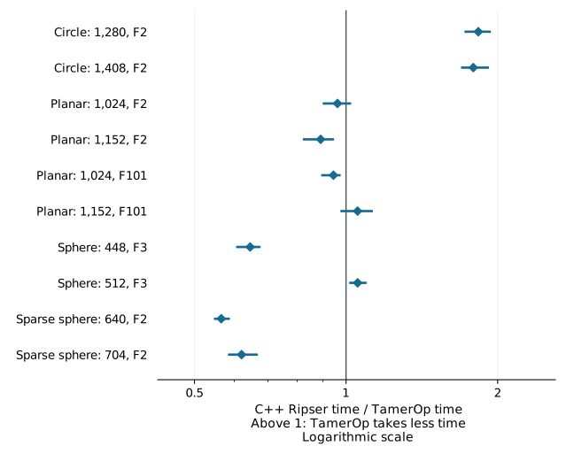
A ratio above one favors TamerOp: a value of 2 means it takes half as long. A ratio below one favors C++ Ripser. Markers average the ratios from three rounds of measurements using a geometric mean; lines span the smallest and largest ratio. These ranges show the observed variation between rounds.
Actual runtimes and input sizes
Times are in seconds. For each input, we average the two timings in each round, then take the middle of those three averages. F₂, F₃ and F₁₀₁ denote arithmetic modulo 2, 3 and 101. A degree label H₂ includes H₀, H₁ and H₂. All ten measured inputs appear below.
| Input | Vertices | Field / through | TamerOp (s) | C++ Ripser (s) | C++ / TamerOp time |
|---|---|---|---|---|---|
| Circle | 1,280 | F₂ / H₁ | 15.5 | 28.6 | 1.83× |
| Circle | 1,408 | F₂ / H₁ | 25.5 | 48.8 | 1.79× |
| Planar | 1,024 | F₂ / H₂ | 31.7 | 28.7 | 0.962× |
| Planar | 1,152 | F₂ / H₂ | 55.4 | 45.7 | 0.890× |
| Planar | 1,024 | F₁₀₁ / H₂ | 38.5 | 37.4 | 0.944× |
| Planar | 1,152 | F₁₀₁ / H₂ | 47.2 | 50.1 | 1.05× |
| Sphere | 448 | F₃ / H₂ | 24.9 | 16.8 | 0.645× |
| Sphere | 512 | F₃ / H₂ | 40.6 | 42.7 | 1.05× |
| Sparse sphere | 640 | F₂ / H₂ | 49.8 | 28.0 | 0.565× |
| Sparse sphere | 704 | F₂ / H₂ | 69.7 | 43.7 | 0.620× |
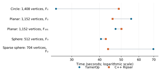
The plot selects the larger input from each family and field. It shows how the ratio translates into elapsed time, including the sparse sphere result favoring C++ Ripser. Reported ratios use the paired process medians. The time columns summarize each program separately, so dividing the displayed times need not give the reported ratio.
What the comparison computes
A Vietoris–Rips filtration adds an edge when its distance reaches the threshold and fills every clique with its simplex. Both programs return the complete barcode through the requested homology degree, including repeated intervals and classes that remain at the end of the filtration. TamerOp uses its direct ordinary persistence route, without constructing a finite encoding.
The inputs contain equally spaced circle points, random planar points in (-1,1)², or normalized Gaussian points on a sphere in R³. Their Euclidean distances are rounded to multiples of 1/4096, which both Float32 and Float64 represent exactly. The benchmark therefore computes persistence on the same supplied dissimilarities in both programs. The input definitions give the sizes, seeds and construction rules.
Sparse inputs retain only edges within the stated radius before either tool reads the graph. A class that remains at the end of such a filtration is essential in that restricted graph; later edges from the full point cloud could kill it. This common restriction matters because a separate small control exposed a cutoff error in this version of C++ Ripser's command line program. The four-vertex example and expected answer record that behavior. It is excluded from speed comparisons.
The Ripser.py report measures a different interface, which adds landmark selection and representative cocycles to its Python workflow. Here the requested result is the barcode alone, from a supplied distance file.
How the measurements were taken
Both programs start from the same text file. The timer includes reading the distances, building the input objects, computing the barcode and printing its intervals. C++ Ripser is launched for every call, and its launch time is included. TamerOp runs in an already loaded Julia session with its code compiled.
We ran three rounds of measurements. Each input starts a new Julia session in each round, with a preliminary run followed by two timed computations per program. Every computation rereads its input and calculates the barcode afresh. Input order reverses in the second round, and the programs alternate going first. The observation record retains the individual timings.
Matching the answers
Complete interval multisets agree by degree, including essential classes and multiplicities. The supplied grades are separated sufficiently that Ripser's printed endpoints decode uniquely to their original values; the harness rejects inputs whose values would become ambiguous when printed. Small controls additionally agree with an independent explicit boundary reduction, covering several fields, equal grades, a stored zero edge and a disconnected sparse component. See the verification record.
Computer, versions and memory
The study used the benchmark computer, with one computation thread per program and one program running at a time. Other work was running on the computer during this study; the plotted ranges show the variation between rounds.
| Component | Recorded version or setting |
|---|---|
| TamerOp | The same frozen source as the Ripser.py study |
| Julia | 1.12.1 |
| C++ Ripser | Upstream commit 01add51ff64aaf40889483260cc5c3b7d0f2a1e7 |
| Compiler | g++ 11.4.0, with optimization enabled |
Julia was configured to reclaim unused memory sooner, and each input ran in a separate Julia session. Earlier attempts without these changes exceeded the memory limit. The configuration record gives the settings and identifies the excluded runs.
TamerOp used more RAM. The largest amount recorded for each input ranged from 3.11 to 5.67 GB for TamerOp, compared with about 25 MB to 2.17 GB for C++ Ripser. These measurements cover the whole program: a Julia session includes setup and repeated computations of one input, while each C++ call runs separately. The data dictionary explains the measurements in the complete table.
Reproduce the results
Follow Reproduce a benchmark report to verify the records and regenerate the common figures. The study's principal files are:
| Record | Download |
|---|---|
| File and field descriptions | Data dictionary |
| Full summary and paired ratios | summary.json · summary.csv |
| Individual observations | observations.json |
| Mathematical checks | verification.json · control checks |
| Inputs and timing protocol | manifest.json · fixtures.json |
| Software, harness and computer | source hashes · harness hashes · machine and build |
| Integrity checks | SHA256SUMS |
The SHA-256 of summary.json is:
0ee767629be22d60dc77760cd654feba76b0983d4b8a512c343166a5dae8607dThe benchmark project provides the frozen TamerOp source, original measurement workers and input generator. Preparation checks out the pinned C++ source, builds its two coefficient variants and verifies the generated input hashes. The reproduction guide walks through checking the published records, rebuilding these figures and running a new comparison on your own machine.