Following vectors and constructing generated submodules
Download the executed notebook · Build and environment record
Suppose we choose a vector in one space of a persistence module and follow it forward. At some parameters its image may be zero even though the surrounding module still has a nonzero space. To understand this vector, we need to apply the maps to its coordinates.
We will follow vectors in two overlapping square supports, then collect their images into a submodule and form the quotient by it. The input is a finite diagram over $\mathbb Q$, supplied directly, with a classifier that lets us view the answer on regions of the parameter plane. You need Julia, TamerOp and CairoMakie, along with vectors and matrix multiplication. The spaces and maps guide gives the surrounding query workflow. OP denotes the main interface; A = OP.Advanced supplies the finite constructors and inclusion and quotient queries used below.
import TamerOp as OP
using CairoMakie
A = OP.Advanced
TamerOp.AdvancedTwo squares and their overlap
The first square is $[0,2)\times[1,3)$ and the second is $[1,3)\times[0,2)$. Each contributes one coordinate wherever it is active. In their overlap the stalk, the vector space at a parameter, is $\mathbb Q^2$ with basis $e_1,e_2$. Along a comparable pair, a coordinate survives exactly when its square is active at both ends. Thus the map from the overlap into the upper arm is $[1\;0]$, and the map into the right arm is $[0\;1]$.
The code records these spaces and maps on a $4\times4$ grid of finite labels. Its first coordinate varies fastest, so label 6 represents the overlap cell $[1,2)\times[1,2)$. These half-open cells include their lower and left boundaries. The classifier assigns labels on the nonnegative quadrant; a point with a negative coordinate is unrepresented. Some represented labels have zero stalks, which is a different situation.
P = A.ProductOfChainsPoset((4, 4))
points = [(x, y) for y in 0:3 for x in 0:3]
active = [findall(identity, [0 <= x < 2 && 1 <= y < 3,
                           1 <= x < 3 && 0 <= y < 2]) for (x, y) in points]
dims = length.(active)
maps = Dict((u, v) => OP.QQ[a == b for a in active[v], b in active[u]]
            for (u, v) in A.cover_edges(P))
M = A.PModule{OP.QQ}(P, dims, maps; field=OP.CoreModules.QQField())
classifier = A.GridEncodingMap(P, (collect(0:3), collect(0:3)))
enc = OP.EncodingResult(P, M, classifier)
OP.describe(enc)
(kind = :encoding_result, poset_type = TamerOp.FiniteFringe.ProductOfChainsPoset{2}, module_type = TamerOp.Modules.PModule{Rational{BigInt}, TamerOp.CoreModules.CoeffFields.QQField, Matrix{Rational{BigInt}}, TamerOp.FiniteFringe.ProductOfChainsPoset{2}}, encoding_map_type = TamerOp.EncodingCore.GridEncodingMap{2, Int64, TamerOp.FiniteFringe.ProductOfChainsPoset{2}}, compiled = false, backend = :auto, has_cohomology = false, has_presentation = false, module_dims = [0, 1, 1, 0, 1, 2, 1, 0, 1, 1, 0, 0, 0, 0, 0, 0], materialized = true, provenance = (category = :finite_poset_representations, base_poset = ProductOfChainsPoset(axes=(4, 4), orientation=(1, 1), nvertices=16), field = TamerOp.CoreModules.CoeffFields.QQField(), degree = nothing, degree_convention = :not_applicable, encoding = (map_type = TamerOp.EncodingCore.GridEncodingMap{2, Int64, TamerOp.FiniteFringe.ProductOfChainsPoset{2}}, backend = :auto), window = :not_recorded, orientation = :not_recorded, construction = (requested = :not_recorded, effective = :not_recorded, substitution = :not_recorded), discretization = :not_recorded, approximation = :not_recorded, backend = (requested = :not_recorded, effective = :auto), ambient_identification = :not_asserted))Follow one vector
Start with $e_1=(1,0)$ at label 6. The first coordinate survives in the upper arm and disappears in the right arm, as the two matrices above predict. source asks for a finite label, and vectors gives coordinates in that stalk's stored basis. The returned propagation result retains the image columns and their ranks, so we can inspect this selection before constructing a module from it.
first_vector = OP.propagate(enc; source=6, vectors=[1, 0])
@assert OP.propagation_summary(first_vector).nonzero_support == [6, 10]
OP.propagation_summary(first_vector)
(kind = :vector_propagation, source = 6, field = TamerOp.CoreModules.CoeffFields.QQField(), basis_convention = :ambient_stalk_coordinates, columns = 1, image_dimensions = Union{Nothing, Int64}[nothing, nothing, nothing, nothing, nothing, 1, 0, 0, nothing, 1, 0, 0, nothing, 0, 0, 0], nonzero_support = [6, 10], applicable_vertices = [6, 7, 8, 10, 11, 12, 14, 15, 16], encoding = EncodingResult(backend=auto, module_type=PModule, compiled=false, materialized=true), exact = true, path_independence = :selected_columns_checked, summand = :not_certified)OP.visualize(first_vector)
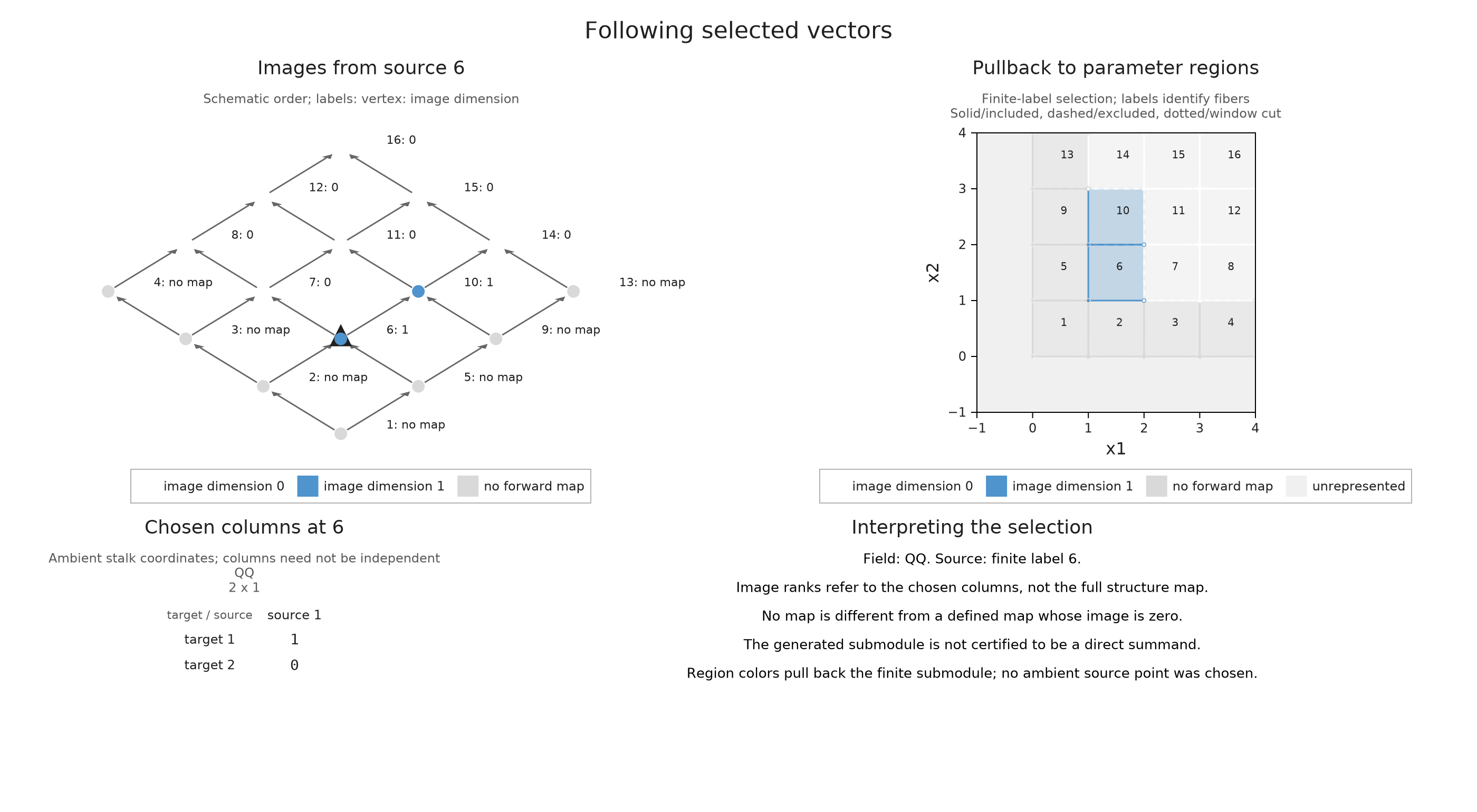
In the figure, a label written q: d has image dimension $d$ at vertex $q$. Only labels 6 and 10 carry a nonzero image of $e_1$. The right arm still has a nonzero ambient stalk, but its matrix $[0\;1]$ annihilates the chosen vector. Labels outside the source's upper ideal, the set of vertices greater than or equal to 6, have no forward map from this source.
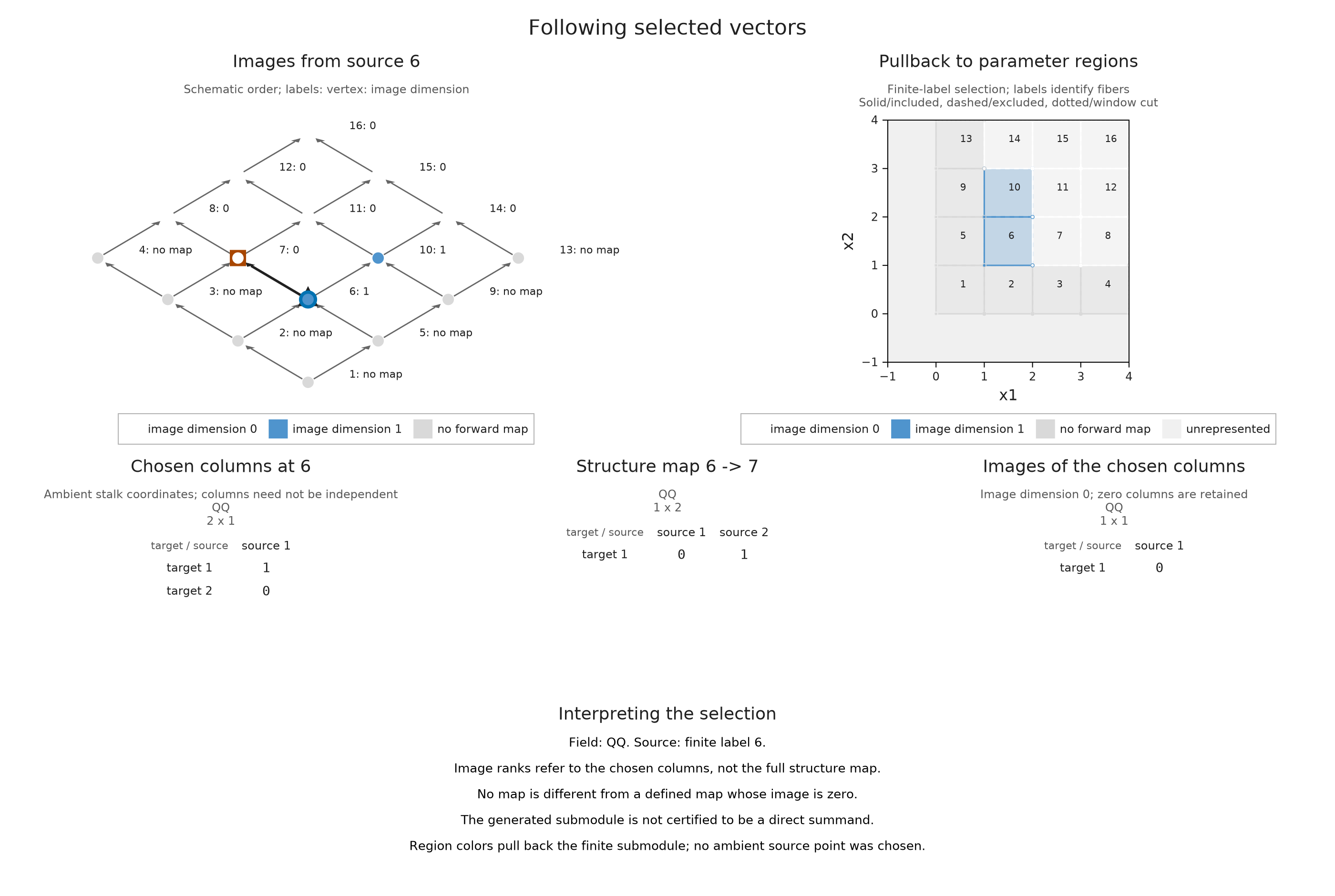
Selecting target 7 displays the matrix and the resulting zero column together. The zero column has one row because the ambient target space is one-dimensional.
OP.visualize(first_vector; target=7)
Change the chosen vector
For $e_2=(0,1)$ the roles of the arms reverse. For $e_1+e_2=(1,1)$, either arm receives the scalar 1. At the overlap, however, we have still chosen only one vector, spanning the diagonal line in a two-dimensional space. Its image dimension there is one.
second_vector = OP.propagate(enc; source=6, vectors=[0, 1])
sum_vector = OP.propagate(enc; source=6, vectors=[1, 1])
@assert OP.propagation_summary(second_vector).nonzero_support == [6, 7]
@assert OP.propagation_summary(sum_vector).nonzero_support == [6, 7, 10]
OP.visualize(sum_vector; target=10)
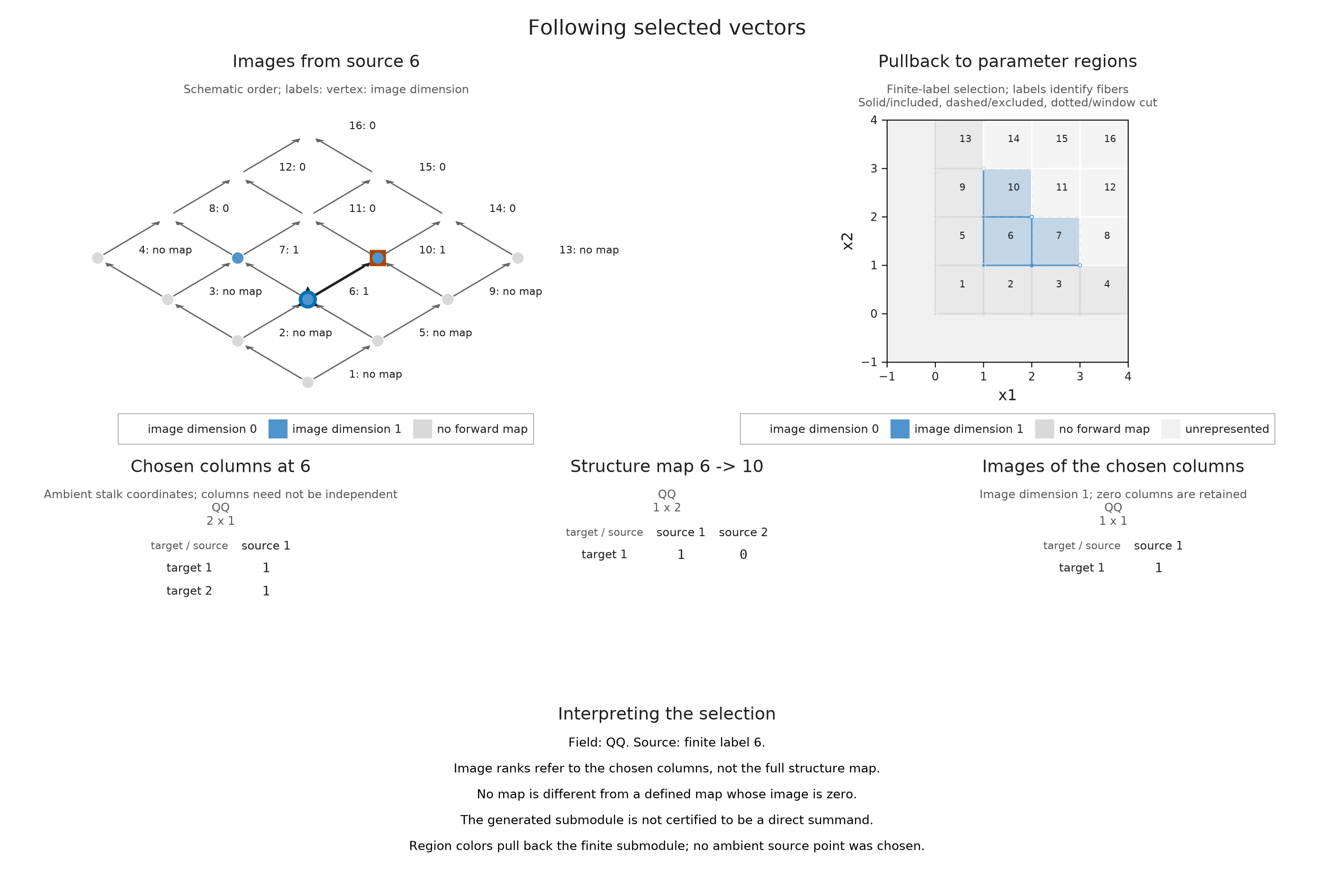
The region panel colors each classifier fiber by the answer at its finite label. We selected label 6 as a whole, rather than a particular original point inside its cell. If we later choose a point in that cell, other points with the same label can lie below it or be incomparable with it. The region picture therefore describes the pullback of a finite submodule; it does not assert that every colored point is reachable from any chosen original point.
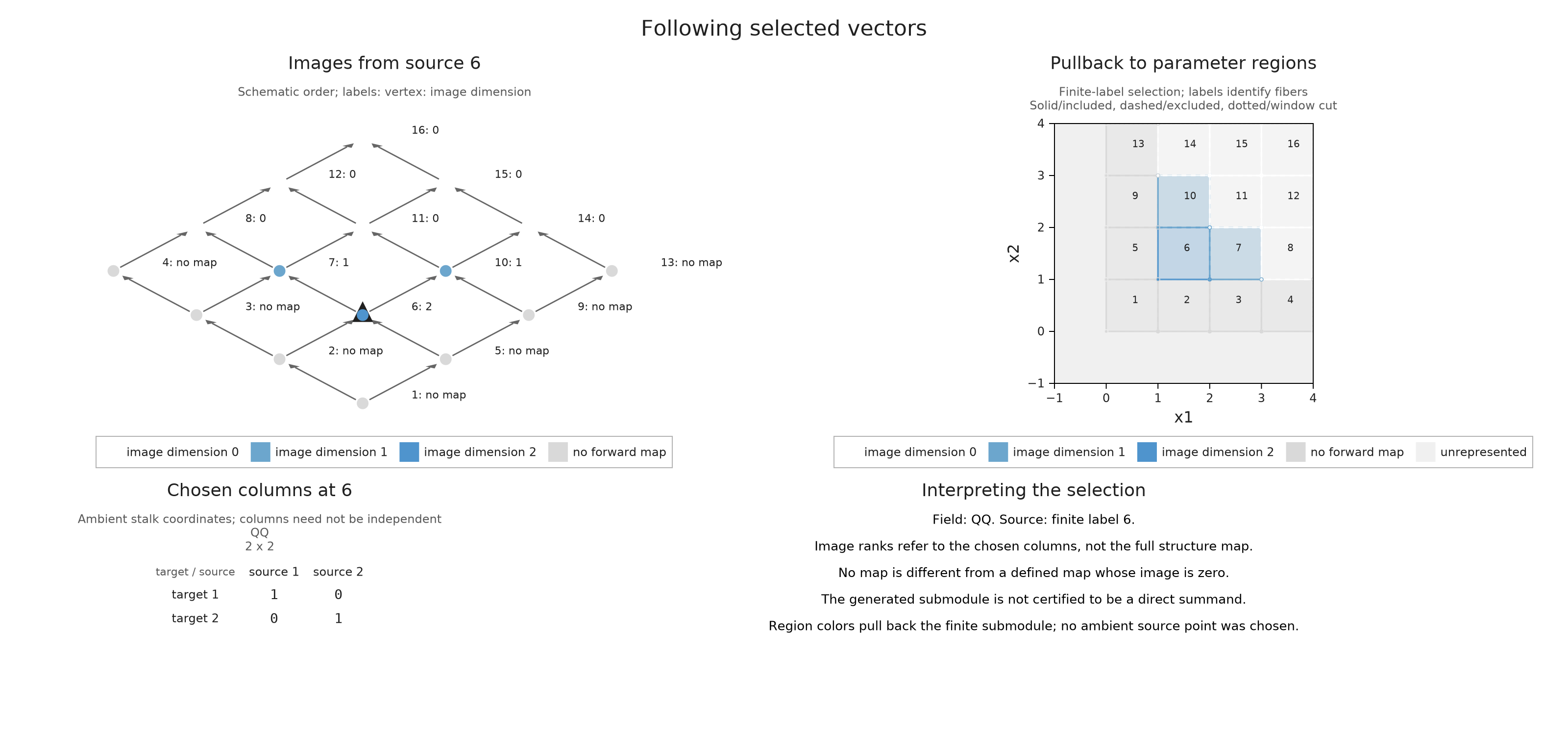
We can select a subspace by supplying spanning columns. The identity matrix selects the whole overlap plane, so its image dimensions are two at label 6 and one along either arm. Dependent columns are accepted too; the dimension is the rank of their images, not the number of supplied columns.
plane = OP.propagate(enc; source=6, vectors=[1 0; 0 1])
@assert OP.dimensions(plane)[6] == 2
@assert OP.dimensions(plane)[7] == 1
OP.visualize(plane; size=(1600, 770))
Compare the vectors at one target
Keep the source at label 6 and the target at label 7, so the map remains $[0\;1]$. Changing the chosen columns shows what this fixed map does to $e_1$, $e_2$, $e_1+e_2$ and the whole overlap plane. The first vector disappears at the target; the other choices have a one dimensional image there. The finite order and region panels show why their generated spaces still differ elsewhere, including dimension two at the source when the whole plane is chosen.
Compare the chosen vectors and their images
Recover the generated submodule
Let $B$ contain our selected columns at a finite source $p$. At a vertex $q\geq p$, take their image span
\[N(q)=\operatorname{im}\bigl(M(p\leq q)B\bigr),\]
and put $N(q)=0$ at all other vertices. This collection is closed under the maps: if $p\leq q\leq r$, applying $M(q\leq r)$ to these images gives $M(p\leq r)B$. Every submodule containing the original columns must contain all these images, so $N$ is the smallest such submodule. It is called the generated submodule.
OP.generated_submodule constructs its spaces and induced maps. The returned S records both this module and its inclusion into the original module. submodule_object(S) gives the module itself; inclusion_map(S) tells us how each of its coordinates sits in the ambient space.
S = OP.generated_submodule(sum_vector)
N = A.submodule_object(S)
inclusion = A.inclusion_map(S)
@assert OP.dimensions(N).stalks == [0, 0, 0, 0, 0, 1, 1, 0, 0, 1, 0, 0, 0, 0, 0, 0]
@assert A.check_submodule(S).valid
OP.describe(S)
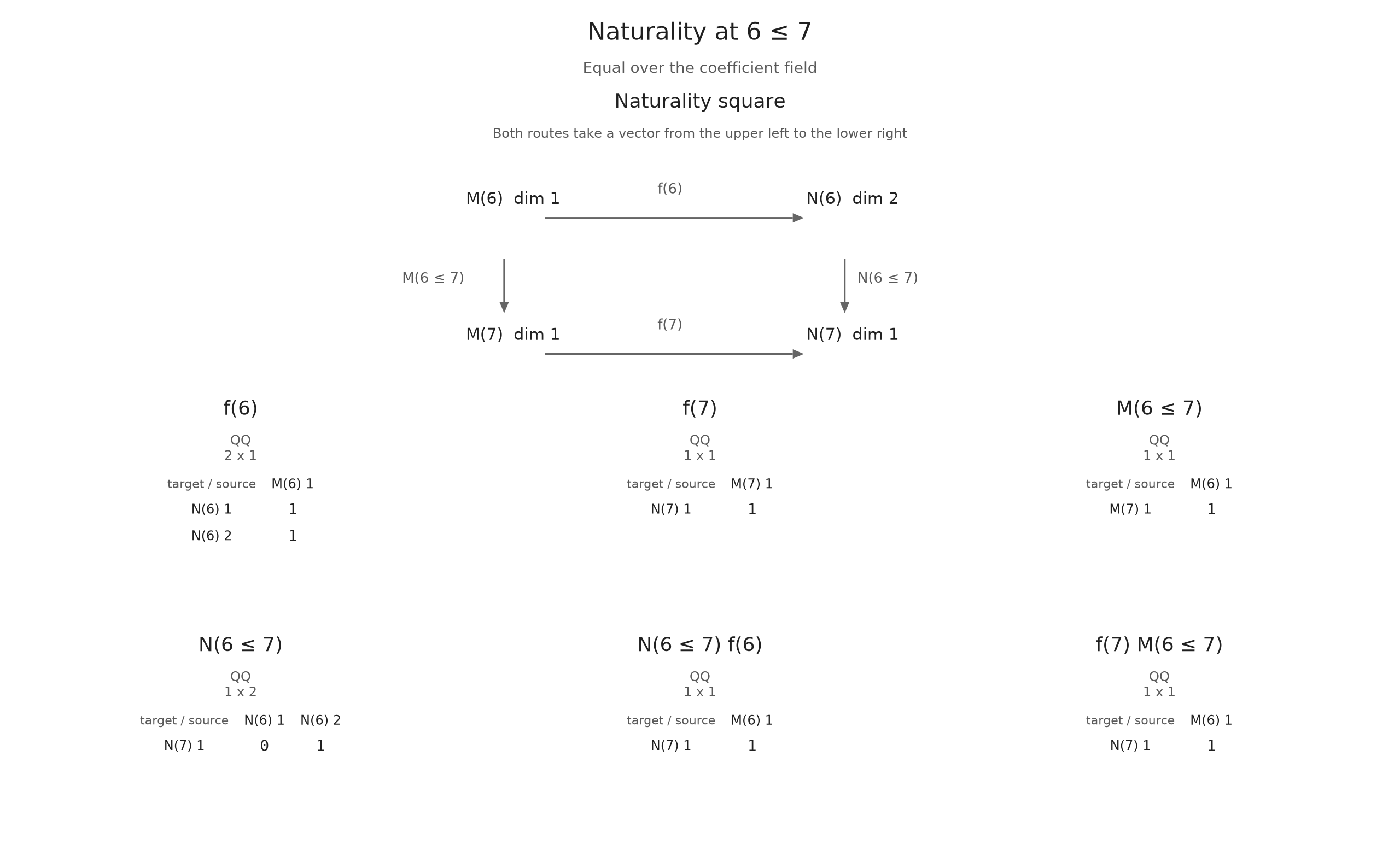
(kind = :submodule, field = "Rational{BigInt}", dimensions = (vertices = 16, submodule = [0, 0, 0, 0, 0, 1, 1, 0, 0, 1, 0, 0, 0, 0, 0, 0], ambient = [0, 1, 1, 0, 1, 2, 1, 0, 1, 1, 0, 0, 0, 0, 0, 0], submodule_total = 3, ambient_total = 8))For our selected sum, $N(6)$ is the line spanned by $(1,1)$, while $N(7)$ and $N(10)$ are one-dimensional. The inclusion is compatible with the maps. For instance, following its vector from 6 to 7 in the ambient module gives $[0\;1](1,1)^{\mathsf T}=1$, just as first following the generated module's map and then including its image does.
The viewer calls its source module M and its target module N; for this figure those are our generated module and ambient module, respectively. The displayed commuting square expresses the compatibility using the actual bases returned by the construction.
OP.visualize(inclusion; kind=:naturality, pair=(6, 7))
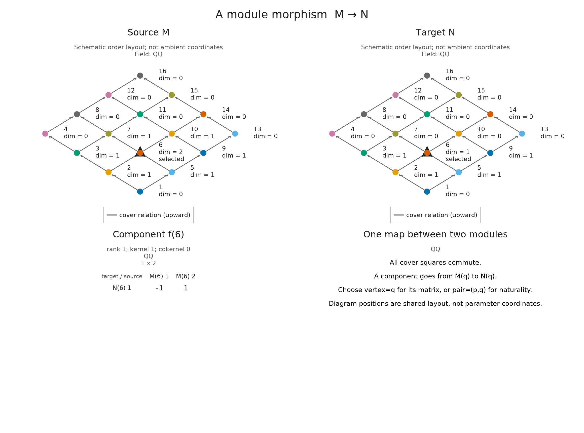
The quotient $M/N$ identifies two ambient vectors when their difference lies in the generated subspace. At the overlap, the diagonal line is removed from $\mathbb Q^2$, leaving a one-dimensional quotient. Either arm is entirely generated, so its quotient is zero.
quotient_with_projection(S) returns both the quotient module and the map sending an ambient vector to its class. This projection must annihilate every included vector. We check that equation at every finite label before inspecting its matrix at label 6. Empty matrices are the expected components where a source or target has dimension zero.
quotient, projection = A.quotient_with_projection(S)
@assert all(iszero(A.component(projection, q) * A.component(inclusion, q)) for q in 1:16)
OP.visualize(projection; vertex=6)
A submodule need not split
It is tempting to think that removing a subspace at each vertex leaves a complementary module inside the original one. The maps can prevent those local complements from fitting together.
Consider the identity map $\mathbb Q\xrightarrow{1}\mathbb Q$ on a chain of two vertices. A vector chosen at the second vertex generates $0\to\mathbb Q$. A complementary submodule would have to be $\mathbb Q\to0$, but the ambient identity carries its first nonzero space outside its proposed second space. There is no such complementary submodule, although the quotient with dimensions $(1,0)$ exists.
chain = A.ProductOfChainsPoset((2,))
constant = A.PModule{OP.QQ}(chain, [1, 1], Dict((1, 2) => ones(OP.QQ, 1, 1)); field=OP.CoreModules.QQField())
tail = OP.generated_submodule(OP.propagate(constant; source=2, vectors=[1]))
@assert OP.dimensions(A.submodule_object(tail)).stalks == [0, 1]
OP.describe(tail)
(kind = :submodule, field = "Rational{BigInt}", dimensions = (vertices = 2, submodule = [0, 1], ambient = [1, 1], submodule_total = 1, ambient_total = 2))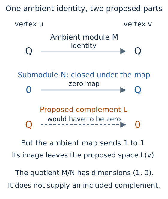
This schematic follows the ambient map on each proposed space. The quotient exists, but its spaces cannot be included as a complementary submodule of this diagram.
What remains unchanged under a basis change?
Replace the two spanning columns of the overlap plane by $(1,1)$ and $(0,1)$. Before running the calculation, predict the image dimensions: the new columns span the same plane, so applying any fixed linear map gives the same image subspace. The matrices of individual columns change, but their image ranks agree.
other_columns = OP.propagate(enc; source=6, vectors=[1 0; 1 1])
@assert OP.dimensions(other_columns) == OP.dimensions(plane)
OP.dimensions(other_columns)
16-element Vector{Union{Nothing, Int64}}:
  nothing
  nothing
  nothing
  nothing
  nothing
 2
 1
 0
  nothing
 1
 0
 0
  nothing
 0
 0
 0
Optional: prepare the vector comparison
Each propagation result already contains the selected columns and their images. We retain the finite order, its parameter regions and the two column matrices so that the browser can compare the choices without constructing another submodule.
vector_labels = ["First vector e1", "Second vector e2", "Diagonal vector e1 + e2", "Whole overlap plane"]
propagations = [first_vector, second_vector, sum_vector, plane]
expected_images = [reshape(OP.QQ[0],1,1), reshape(OP.QQ[1],1,1),
                   reshape(OP.QQ[1],1,1), OP.QQ[0 1]]
vector_views = []
for (label, propagation, expected) in zip(vector_labels, propagations, expected_images)
    @assert A.propagation_image(propagation; target=7) == expected
    answer = A.visual_spec(propagation; target=7)
    push!(vector_views, OP.compose_visuals((
        regions=OP.visual_panel(answer; panel=:propagation_regions),
        order=OP.visual_panel(answer; panel=:propagation_hasse),
        columns=OP.visual_panel(answer; panel=3),
        images=OP.visual_panel(answer; panel=5));
        columns=2, title=label, subtitle="Source label 6; target label 7; structure map [0 1] over Q."))
end
prepared_vectors = NamedTuple{Tuple(Symbol.(vector_labels))}(Tuple(vector_views))
submodule_directory = joinpath("tamerop_outputs", "submodules")
mkpath(submodule_directory)
OP.save_visual_session(joinpath(submodule_directory, "vectors.html"), prepared_vectors;
    selected=Symbol("First vector e1"), size=(1400,1000),
    title="Change the selected vectors while keeping the map fixed",
    caption="The map from Q squared at label 6 to Q at label 7 is [0 1]. Region colors give image dimensions on the half open classifier cells; the finite source is a whole label.");
Changing the ambient stalk bases requires a further step: transform the structure matrices and selected coordinates together. Keeping the same numbers for a vector after changing its ambient basis usually selects a different vector.
For the finite diagram here, the coordinate spaces are the input, so the images and inclusion answer the question completely. When a module came from homology, we may instead want to recognize the selected image as a cycle in the original complex. The optional section below explains what additional basis information that requires.
The module reference gives accepted shapes and field conventions. To follow how the image spans become a module with maps, continue with the implementation account.
Relate an image to source cycles
For a homology module with retained cycles, A.propagation_source_chain(result; target, basis, column=1) expresses a propagated column on the original cells. Supply the ordered homology basis corresponding to the actual target coordinates. The routine checks that these are cycles and that they form a basis modulo boundaries; the identification with the module's coordinates is supplied by you. It cannot recover a discarded basis. The returned SourceChain can be explored using the source cell views.
You can inspect the generated module itself through OP.inspection_session(N), using the live inspection guide for controls. Changing which vectors you want to follow starts a fresh OP.propagate computation.