Reading scalar fields in their original coordinates
Download the executed notebook · Build and environment record
A numerical feature retains a chosen part of a module's information, such as the height of a persistence landscape at a parameter. A picture can help us read those values once we know where they belong: which coordinates are being shown, which coordinates are fixed, and which landscape layer or other scalar function supplies the colors.
We begin with a module supported on a square, whose landscape we can predict. We will place sampled line landscapes back in the parameter plane, then use the same viewing operations for sections of a field with four coordinates. You need TamerOp, CairoMakie, basic arrays and the idea of a finite encoding. The ordinary analysis guide introduces landscapes of barcodes; the API reference gives the precise controls.
import TamerOp as OP
using CairoMakie
const A = OP.Advanced
const QQ = Rational{BigInt}
Rational{BigInt}A rectangle gives a landscape we can check
Take the module that has one copy of the rational field on $[0,4)\times[0,4)$ and zero elsewhere on the nonnegative plane, with identity maps inside the square. Four finite labels suffice for this encoding: only the first carries a nonzero space. The encoding map assigns each parameter its label using the thresholds 0 and 4.
A barcode interval gives a tent whose height is the distance to its nearer endpoint. Along a diagonal through $(x,y)$ inside the square, we can move the same distance in both directions before meeting a side. The largest such distance is $\min(x,y,4-x,4-y)$, which is the first diagonal landscape height. The second layer is zero because every slice has at most one interval. This gives us a formula to compare with the computation.
P = A.ProductOfChainsPoset((2,2))
dims = [1,0,0,0]
maps = Dict(e => zeros(QQ,dims[e[2]],dims[e[1]]) for e in A.cover_edges(P))
M = A.PModule{QQ}(P,dims,maps;field=OP.CoreModules.QQField())
pi = A.GridEncodingMap(P,([0,4],[0,4]))
enc = OP.EncodingResult(P,M,pi)
OP.describe(enc)
(kind = :encoding_result, poset_type = TamerOp.FiniteFringe.ProductOfChainsPoset{2}, module_type = TamerOp.Modules.PModule{Rational{BigInt}, TamerOp.CoreModules.CoeffFields.QQField, Matrix{Rational{BigInt}}, TamerOp.FiniteFringe.ProductOfChainsPoset{2}}, encoding_map_type = TamerOp.EncodingCore.GridEncodingMap{2, Int64, TamerOp.FiniteFringe.ProductOfChainsPoset{2}}, compiled = false, backend = :auto, has_cohomology = false, has_presentation = false, module_dims = [1, 0, 0, 0], materialized = true, provenance = (category = :finite_poset_representations, base_poset = ProductOfChainsPoset(axes=(2, 2), orientation=(1, 1), nvertices=4), field = TamerOp.CoreModules.CoeffFields.QQField(), degree = nothing, degree_convention = :not_applicable, encoding = (map_type = TamerOp.EncodingCore.GridEncodingMap{2, Int64, TamerOp.FiniteFringe.ProductOfChainsPoset{2}}, backend = :auto), window = :not_recorded, orientation = :not_recorded, construction = (requested = :not_recorded, effective = :not_recorded, substitution = :not_recorded), discretization = :not_recorded, approximation = :not_recorded, backend = (requested = :not_recorded, effective = :auto), ambient_identification = :not_asserted))The landscape workflow normalizes our requested diagonal direction $(1,1)$ to $(1/2,1/2)$, so the stored line through the basepoint $(0,b)$ is $x(t)=(0,b)+t(1/2,1/2)$. Increasing $t$ by two increases each ambient coordinate by one. The tent height measured in $t$ must therefore be halved when we express it in the original diagonal units.
We supply a common parameter window and evaluation times separated by $1/2$. The barcode calculation determines where the line crosses the encoding regions; evaluating its landscape on tgrid is a subsequent sampling choice.
offsets = collect(-4.:0.5:4.)
tgrid = collect(-8.:0.5:16.)
L = OP.mp_landscape(enc; directions=[[1.,1.]], offsets=[(0.,b) for b in offsets],
    tgrid=tgrid, ts=tgrid, kmax=2)
OP.mp_landscape_summary(L)
(kind = :mp_landscape, ndirections = 1, noffsets = 17, kmax = 2, grid_length = 49, values_shape = (1, 17, 2, 49), weight_shape = (1, 17), total_weight = 1.0, t_range = (-8.0, 16.0), weights_normalized = true)Put each sample where it belongs
ambient_landscape uses the actual basepoints to locate samples in the parameter plane and rescales their heights using the stored direction. It interpolates between consecutive times on a stored line. A point on an unstored line remains unavailable, because these samples alone provide no interpolation between lines. Slice weights, which are useful when averaging or integrating features, do not change the height at a point.
For this square the tent corners fall on our sample times, so we can compare the first layer with its formula on the entire requested grid. We set sample_error=0 because the retained samples have those known values. The reported interpolation bound concerns this line landscape and the declared sample error; earlier approximations to an input or statistical uncertainty would need their own analysis.
grid = collect(0.:0.5:4.)
g = OP.ambient_landscape(L; axes=(grid,grid), basepoints=[(0.,b) for b in offsets],
    source_window=(-8.,16.), sample_error=0.)
expected = [max(0.,min(x,y,4-x,4-y)) for x in grid,y in grid]
@assert A.landscape_values(g)[:,:,1] ≈ expected
@assert all(iszero,A.landscape_values(g)[:,:,2])
f = OP.ScalarField(g;id="Square module",axis_labels=("x","y"))
OP.visualize(f;layer="1",contours=[0.5,1.,1.5])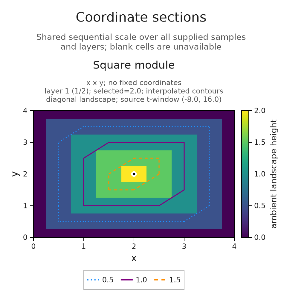
The highest point occurs at the center $(2,2)$, where we can move distance two along either diagonal direction before leaving the square. Contours join equal values in the piecewise affine interpolation of the samples. They help us follow a landscape height, while the square's support boundary remains specified by the original encoding.
The next view selects layer 2 and preserves the color scale across layers. Since every slice has only one interval, the zero panel is the expected mathematical answer.
The prepared viewer below lets you switch between these layers while keeping the selected point at $(2,2)$ and the color scale fixed from 0 to 2. Watch the peak disappear in layer 2: a zero value records the absence of a second interval along the line.
OP.visualize(f;layer="2")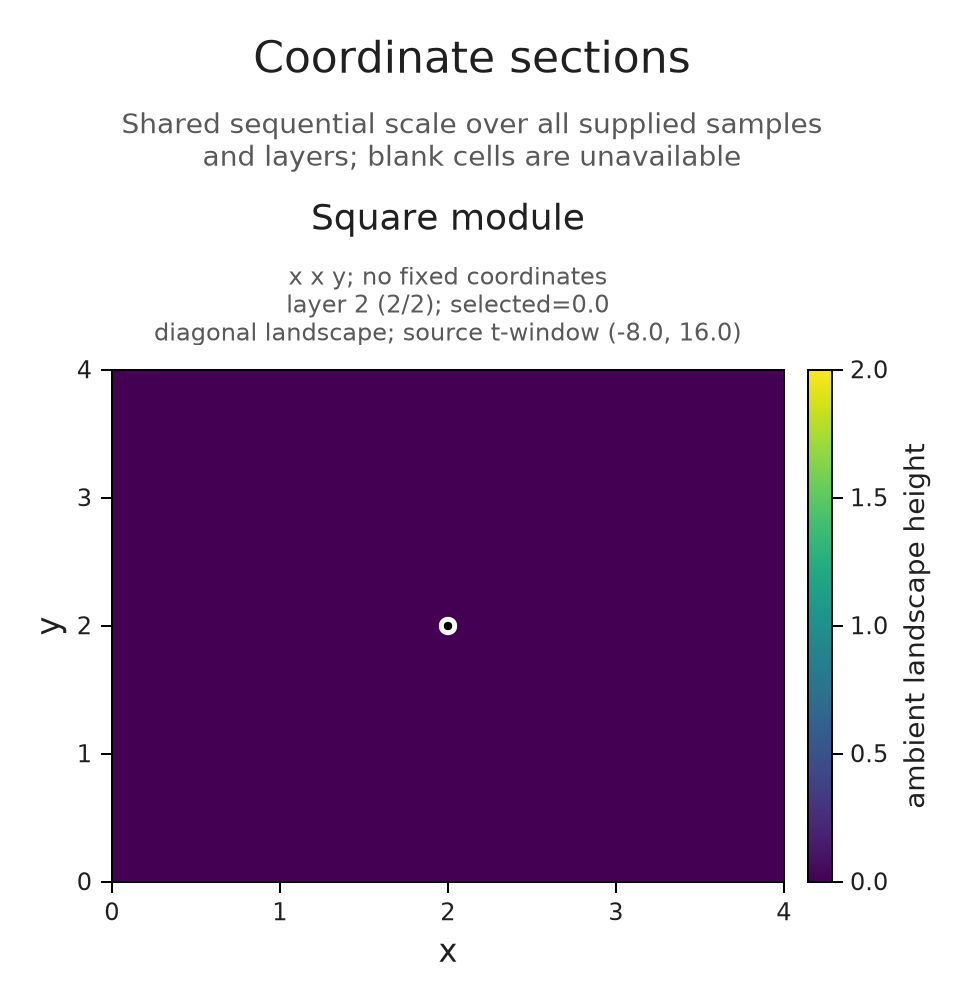
A plane inside four coordinates
The same viewing operations apply to other scalar functions sampled on a Cartesian grid, a set containing every combination of the supplied coordinate values. We use $F(a,b,c,d)=a+2b-c+d$ so we can check the section directly. ScalarField records the axes and their values; it does not infer a module behind them.
To draw a plane, choose two coordinates to vary and fix the others at a selected point. The first panel uses $c$ horizontally and $a$ vertically, holding $b=0$ and $d=9$. The second uses $b$ horizontally and $d$ vertically, holding $a=2$ and $c=30$. Both show sections through the same point.
axes4 = ([2.,5.],[-3.,0.,4.],[10.,20.,30.,40.],[7.,9.])
values = [a+2b-c+d for a in axes4[1],b in axes4[2],c in axes4[3],d in axes4[4]]
field = OP.ScalarField(axes4,values;id="F",axis_labels=("a","b","c","d"),units="response")
session = OP.field_session(field;planes=[(3,1),(2,4)],indices=(1,2,3,2),contours=[-20.,-10.,0.])
OP.visualize(A.inspection_snapshot(session))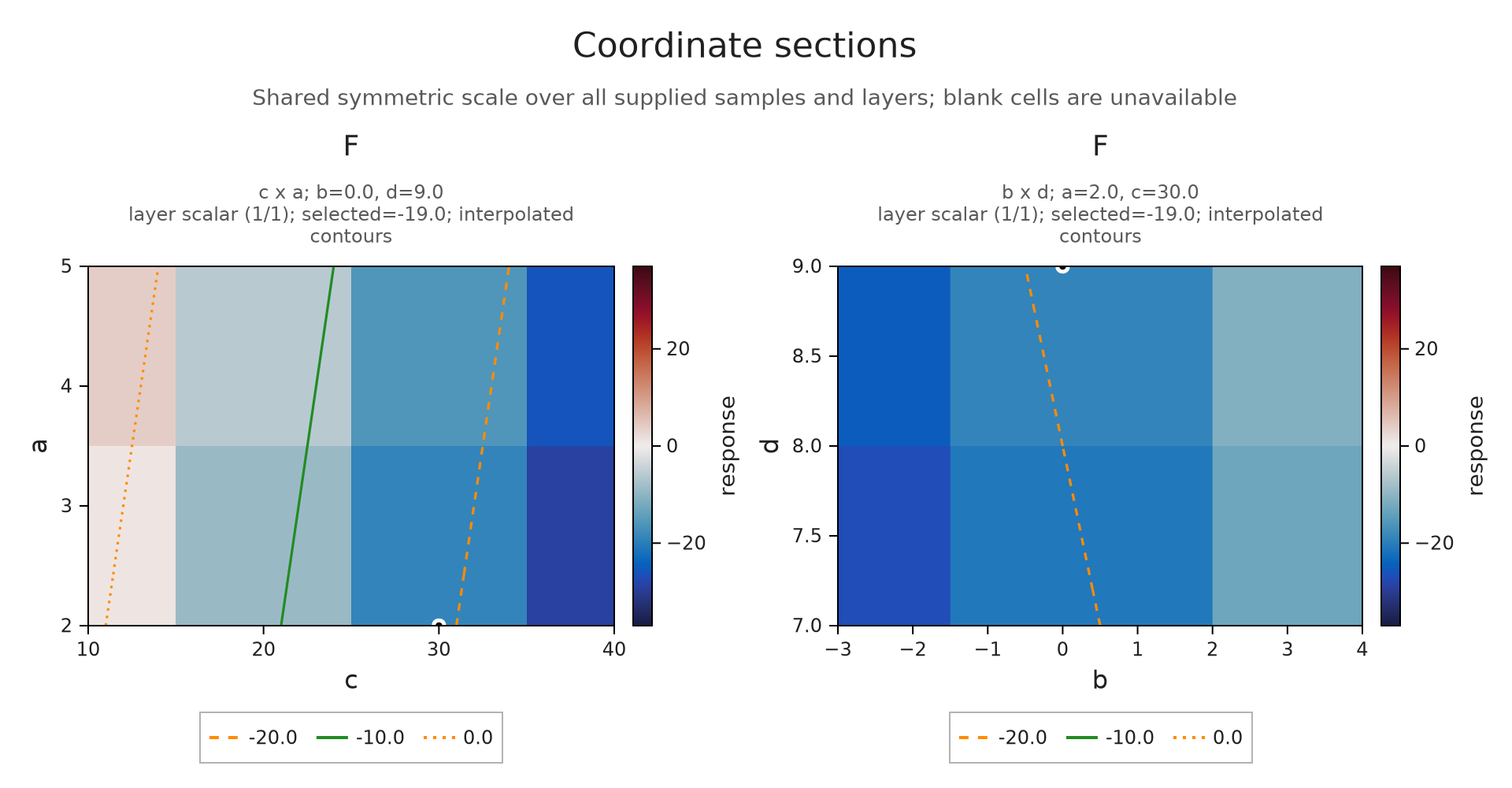
At $(a,b,c,d)=(2,0,30,9)$, the displayed value should be $2+0-30+9=-19$. Changing $b$ from 0 to 4 adds eight, giving $-11$. In the first plane this changes a fixed coordinate and hence the whole section. In the second plane it moves the selected point along an axis already shown. The shared color scale stays fixed, allowing those two effects to be compared.
The linked viewer keeps four selections ready to compare. Begin with b = 0 and b = 4 to follow this change. Its two remaining choices use $(5,-3,20,7)$ and exchange the horizontal and vertical axes of the first panel; both should give the value $-14$. The coordinate labels and fixed color scale let us separate a change of section from a change in how the same section is drawn.
@assert all(row.value == -19 for row in A.inspection_summary(session).selected_values)
scale_before = A.inspection_summary(session).scale
A.select_inspection!(session;indices=(1,3,3,2))
@assert all(row.value == -11 for row in A.inspection_summary(session).selected_values)
@assert A.inspection_summary(session).scale == scale_before
OP.visualize(A.inspection_snapshot(session))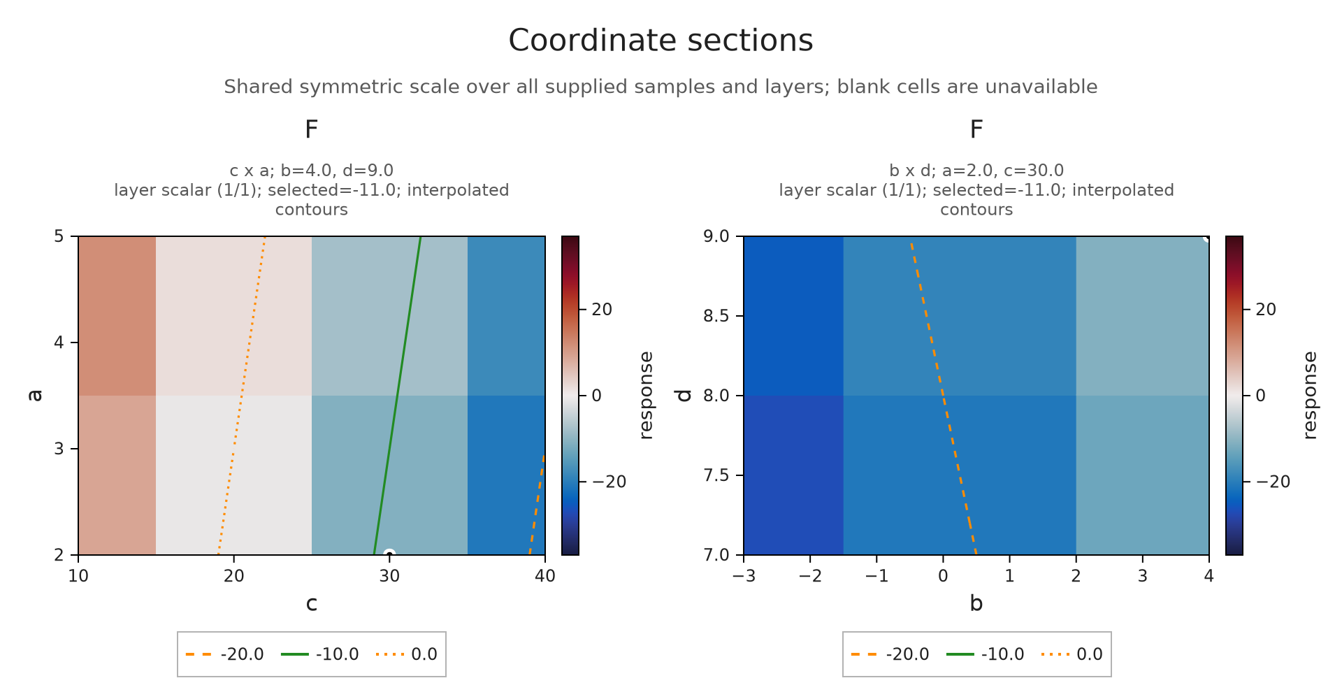
Explore the prepared coordinate sections
Compare values through a declared correspondence
When we pass several fields together, their identical axes, labels, units and ordered layers declare what corresponds. The field IDs keep the individual results identifiable as we move between sections. If results instead use unrelated finite labels, the comparison guide shows how to specify a correspondence between their queries.
Here $G=F+3$. Subtracting the baseline $F$ therefore gives zero for $F$ and three for $G$ at every available sample. A common color scale centered at zero makes both differences readable. If a sample were missing in either field, its difference would remain unavailable.
other = OP.ScalarField(axes4,values .+ 3;id="G",axis_labels=("a","b","c","d"),units="response")
comparison = OP.field_session([field,other];planes=[(3,1)],indices=(1,2,3,2),baseline="F")
@assert A.inspection_summary(comparison).scale.limits == (-3.,3.)
OP.visualize(A.inspection_snapshot(comparison))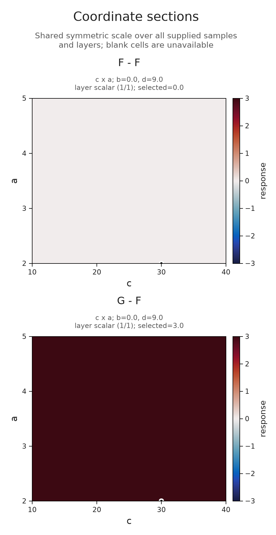
Try another section
Change the selected plane to $(d,b)$ and predict the selected value at $(a,b,c,d)=(5,-3,20,7)$. Does exchanging the horizontal and vertical axes change the scalar answer?
A.select_inspection!(session;planes=[(4,2)],indices=(2,1,2,1))
@assert only(A.inspection_summary(session).selected_values).value == -14
A.select_inspection!(session;planes=[(2,4)])
@assert only(A.inspection_summary(session).selected_values).value == -14
A.inspection_selection(session)
(planes = ((2, 4),), indices = (2, 1, 2, 1), layer = "scalar", normalization = :auto, colorrange = nothing, contours = (-20.0, -10.0, 0.0), baseline = nothing, max_cells = 250000, revision = 3)Optional: query a barcode through a selected point
A scalar field supplies sampled values, while a slice barcode needs the module's structure maps. We can use the field to choose a point and then return to the original encoding for that calculation. Consider a cube module with one copy of the field on $[0,4)^3$ and zero elsewhere in its represented nonnegative domain.
Through $(1,2,3)$, the line $x(t)=(1,2,3)+t(1,1,1)$ enters the cube at $t=-1$ and leaves it at $t=1$. We therefore expect one interval $[-1,1)$. This direct slice query uses the supplied direction $(1,1,1)$, so the returned endpoints are in that line's parameter, without the initial direction normalization used by mp_landscape.
P3 = A.ProductOfChainsPoset((2,2,2))
dims3 = [1; zeros(Int,7)]
maps3 = Dict(e => zeros(QQ,dims3[e[2]],dims3[e[1]]) for e in A.cover_edges(P3))
M3 = A.PModule{QQ}(P3,dims3,maps3;field=OP.CoreModules.QQField())
pi3 = A.GridEncodingMap(P3,([0,4],[0,4],[0,4]))
enc3 = OP.EncodingResult(P3,M3,pi3)
grid3 = collect(0.:4.)
dimensions3 = [dims3[A.locate(pi3,(x,y,z))] for x in grid3,y in grid3,z in grid3]
cube = OP.ScalarField((grid3,grid3,grid3),dimensions3;id="Cube dimensions",units="dimension")
cube_session = OP.field_session(cube;indices=(2,3,4))
selected = Tuple(grid3[i] for i in A.inspection_selection(cube_session).indices)
bars = OP.slice_barcode(enc3;directions=[[1.,1.,1.]],offsets=[selected],ts=collect(-4.:4.))
@assert bars == Dict((-1.,1.)=>1)
A.close_inspection!(cube_session)
OP.visualize(bars;kind=:barcode)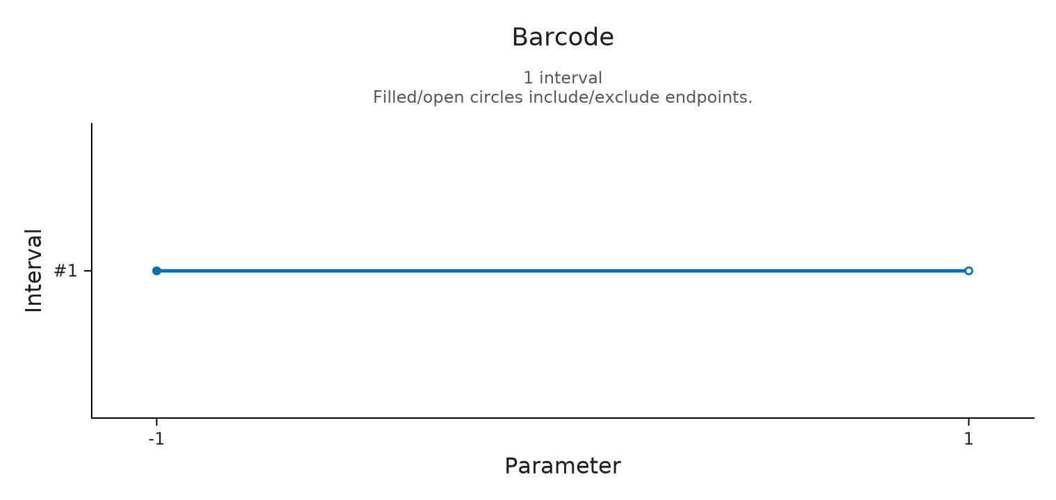
Optional: distinguish a hole in sampling from zero
Suppose we retain only the central diagonal. The samples determine landscape values along that line, including its zero values at the boundary. They provide no values elsewhere in the plane. The next figure preserves this distinction with an availability mask instead of filling the remaining positions by interpolation between lines.
middle = findfirst(==(0.),offsets)
one_line = A.MPLandscape(2,copy(tgrid),copy(L.values[:,middle:middle,:,:]),ones(1,1),copy(A.slice_directions(L)),[(0.,0.)])
sparse_grid = OP.ambient_landscape(one_line;axes=(grid,grid),basepoints=[(0.,0.)],source_window=(-8.,16.))
@assert OP.describe(sparse_grid).covered == length(grid)
sparse_field = OP.ScalarField(sparse_grid; id="One sampled diagonal", axis_labels=("x","y"))
OP.visualize(sparse_field)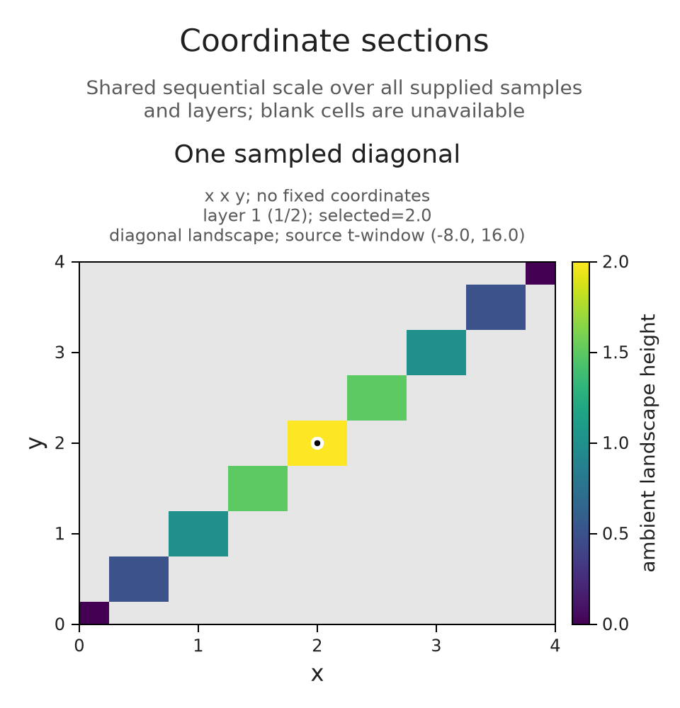
Optional: open the linked controls
With WGLMakie loaded, OP.visualize(session; backend=:wglmakie) opens linked controls while Julia is running. Coordinate sliders and plane or layer choices update each view of the same session. A chart click selects the nearest stored grid point, so the readout still refers to a computed sample. Use the index controls when a particular stored point matters.
A static snapshot retains the fixed coordinates and scale for the selected view. The session guide explains the supported live display paths and how to export selection among saved states; those saved states do not evaluate new queries after Julia closes.
Optional: save the prepared field views
These files keep the layer and section choices used above. We prepare them from the same sampled fields, so changing a browser selection does not evaluate another landscape or alter its sampling. The section figures keep a common color range over the whole field.
layer_views = Pair{Symbol,Any}[]
for layer in ("1", "2")
    selected_layer = OP.Advanced.visual_spec(f; layer, indices=(5,5))
    @assert selected_layer.metadata.scale.limits == (0.,2.)
    @assert only(selected_layer.metadata.selected_values).value == (layer == "1" ? 2. : 0.)
    figure = OP.compose_visuals((landscape=OP.visual_panel(selected_layer),);
        columns=1, title="Landscape layer $layer",
        subtitle="The selected point is (2,2); both layers use the same height scale.")
    push!(layer_views, Symbol("Layer $layer at (2,2)") => figure)
end
layer_viewer_path = joinpath("tamerop_outputs", "features", "layers.html")
mkpath(dirname(layer_viewer_path))
OP.save_visual_session(layer_viewer_path,
    (; layer_views...); title="Choose a landscape layer",
    caption="The square module has rational coefficients. Every sampled line has at most one interval, so layer 2 is zero. Both views use the same original coordinates and height scale from 0 to 2.",
    style=OP.VisualStyle(fontsize=18), size=(760,560));
section_choices = (
    (name="b = 0: value -19", indices=(1,2,3,2), planes=[(3,1),(2,4)], value=-19),
    (name="b = 4: value -11", indices=(1,3,3,2), planes=[(3,1),(2,4)], value=-11),
    (name="d horizontal: value -14", indices=(2,1,2,1), planes=[(4,2),(3,1)], value=-14),
    (name="b horizontal: value -14", indices=(2,1,2,1), planes=[(2,4),(3,1)], value=-14))
section_views = Pair{Symbol,Any}[]
for choice in section_choices
    selected_section = OP.Advanced.visual_spec(field; planes=choice.planes,
        indices=choice.indices, contours=[-20.,-10.,0.])
    @assert selected_section.metadata.scale.limits == (-37.,37.)
    @assert all(row.value == choice.value for row in selected_section.metadata.selected_values)
    push!(section_views, Symbol(choice.name) => selected_section)
end
section_viewer_path = joinpath("tamerop_outputs", "features", "sections.html")
mkpath(dirname(section_viewer_path))
OP.save_visual_session(section_viewer_path,
    (; section_views...); title="Follow a point through coordinate sections",
    caption="F(a,b,c,d) = a + 2b - c + d. Each panel varies its two labelled coordinates and fixes the others at the selected point. Changing b from 0 to 4 adds 8; exchanging the axes changes the drawing but preserves the selected value. Contours interpolate the sampled values.",
    style=OP.VisualStyle(fontsize=18), size=(1100,620));
final_view = A.inspection_snapshot(session)
A.close_inspection!(session)
A.close_inspection!(comparison)
@assert A.inspection_summary(session).closed
@assert A.check_visual_spec(final_view).valid
nothing
We can now read a field value together with its original coordinates, fixed section and layer, including whether a value is available at all. To compare several results through shared queries or named features, continue with comparisons and collections. The landscape implementation account derives the parameter conversion and interpolation bound used here.