Comparing results through declared correspondences
Download the executed notebook · Build and environment record
A change of coefficient field, finite grid or homology degree may change what a figure tells us. To interpret the difference, we first need to identify the questions being compared. We will follow one linear map through two fields and two choices of basis, then compare queries in different finite descriptions of the same parameter domain. This gives us examples where an observable changes, where its coordinates change, and where the query itself changes.
You need TamerOp, CairoMakie and familiarity with spaces and maps. The finite encoding lesson supplies the language for the grid example. The visualization reference gives the complete call contracts, and the implementation account explains how the views reuse prepared results.
The later section on samples and named features begins with a different unit of comparison: a row represents a whole sample. You can enter there if you already have feature or distance tables.
import TamerOp as OP
import CairoMakie
using SparseArrays: sparse

P = OP.Advanced.FinitePoset(BitMatrix([true true; false true]))
F2, F3 = OP.CoreModules.F2(), OP.CoreModules.F3()
K2, K3 = OP.CoreModules.coeff_type(F2), OP.CoreModules.coeff_type(F3)
M2 = OP.Advanced.PModule{K2}(P, [2,2], Dict((1,2) => K2[1 1; 1 -1]); field=F2)
M3 = OP.Advanced.PModule{K3}(P, [2,2], Dict((1,2) => K3[1 1; 1 -1]); field=F3);
Change the field, keep the question
Both modules below have spaces of dimension two at source and target. Their map comes from the integer matrix
\[A=\begin{pmatrix}1&1\\1&-1\end{pmatrix}.\]
Over $\mathbf F_2$, reduction modulo 2 makes the two columns equal, so the image has dimension one. Over $\mathbf F_3$, the determinant $-2$ remains nonzero, so the image has dimension two. The stalk dimensions agree even though these map ranks differ.
ComparisonCase records the construction and its mathematical context. The coefficient field comes from the result itself. Since we supplied a module directly, there is no homology degree to specify. Each list in vertices identifies the source and target queries, and correspondence explains why they should be compared.
fields = OP.compare_visuals((
    f2 = OP.ComparisonCase(M2; filtration="source then target", construction="integer A modulo 2", approximation="exact"),
    f3 = OP.ComparisonCase(M3; filtration="source then target", construction="integer A modulo 3", approximation="exact"));
    vertices=(f2=[1,2], f3=[1,2]),
    correspondence="Source corresponds to source; target to target of the same integral map")
OP.visualize(fields)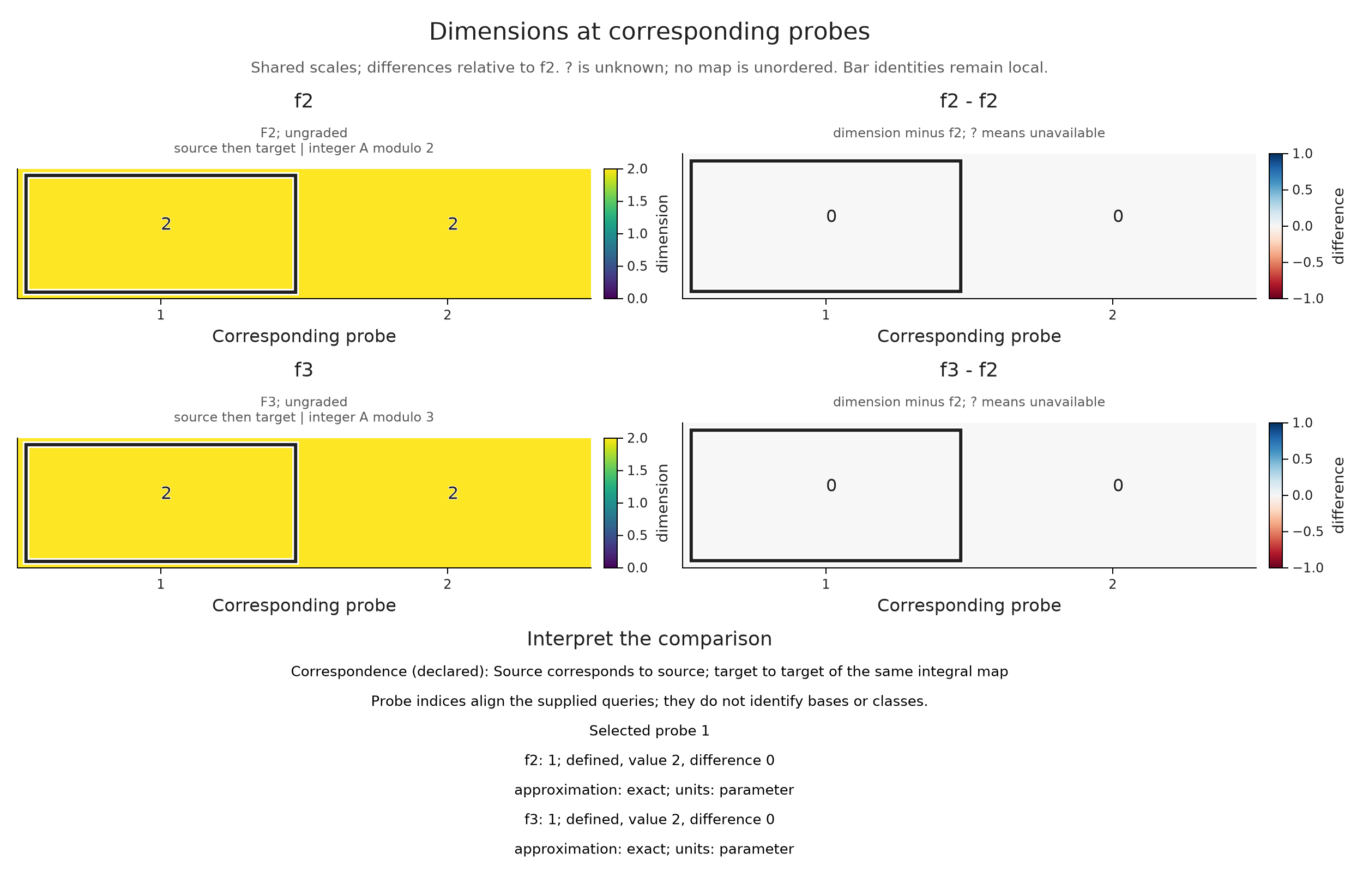
The horizontal positions are query indices: 1 is the source and 2 is the target. The left column gives each dimension, and the right column subtracts the selected baseline. Labels retain the exact numbers alongside the colors.
Now choose view=:rank to follow the map from a fixed source to each query. The source defaults to index 1. Its identity map has rank two over either field, while the map to index 2 has the ranks one and two predicted from the determinant. The comparison makes visible the information that the dimension panels left unanswered.
Use the prepared comparison below to move from the source identity to the target map. At the target, changing the baseline from $\mathbf F_2$ to $\mathbf F_3$ reverses the sign of the nonzero difference. It leaves the two ranks unchanged. The matrices show the selected maps in their stored bases.
rank_view = OP.Advanced.visual_spec(fields; view=:rank, probe=2)
@assert [v.value for v in rank_view.metadata.values.f2] == [2,1]
@assert [v.value for v in rank_view.metadata.values.f3] == [2,2]
OP.visualize(rank_view)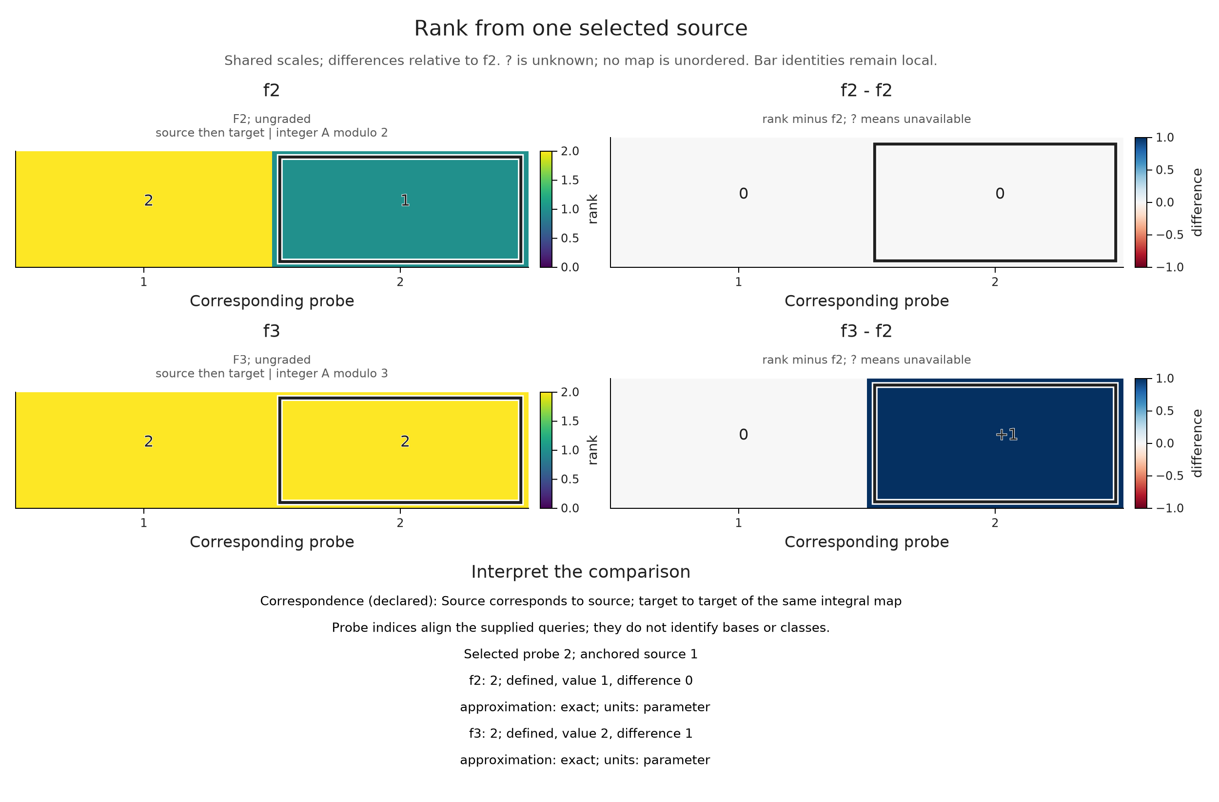
Explore the selected map and baseline
Change coordinates, preserve the map
The same linear map can have different matrices when its source and target bases change. Over $\mathbf Q$, take $A=\left(\begin{smallmatrix}1&0\\0&0\end{smallmatrix}\right)$ and $B=\left(\begin{smallmatrix}1&-1\\1&-1\end{smallmatrix}\right)$. The invertible matrices $S$ at the source and $T$ at the target satisfy $BS=TA$. Following a vector first through the source change and then through $B$ therefore gives the same result as following it through $A$ and then the target change. These two components define an isomorphism of the modules.
We check the equation in rational arithmetic below. The comparison then shows the equal ranks beside the different matrices. Its descriptive correspondence text records our intended interpretation; the matrix equation is what establishes the isomorphism.
A = OP.QQ[1 0; 0 0]
B = OP.QQ[1 -1; 1 -1]
S = OP.QQ[1 1; 0 1]
T = OP.QQ[1 0; 1 1]
@assert B*S == T*A
original = OP.Advanced.PModule{OP.QQ}(P, [2,2], Dict((1,2)=>A); field=OP.CoreModules.QQField())
changed = OP.Advanced.PModule{OP.QQ}(P, [2,2], Dict((1,2)=>B); field=OP.CoreModules.QQField());
bases = OP.compare_visuals((
original=OP.ComparisonCase(original; filtration="source then target", construction="matrix A", approximation="exact"),
changed=OP.ComparisonCase(changed; filtration="source then target", construction="matrix B", approximation="exact"));
vertices=(original=[1,2], changed=[1,2]), correspondence="Specified invertible S and T satisfy B*S=T*A")
OP.visualize(bases; view=:rank, probe=2, matrix=true)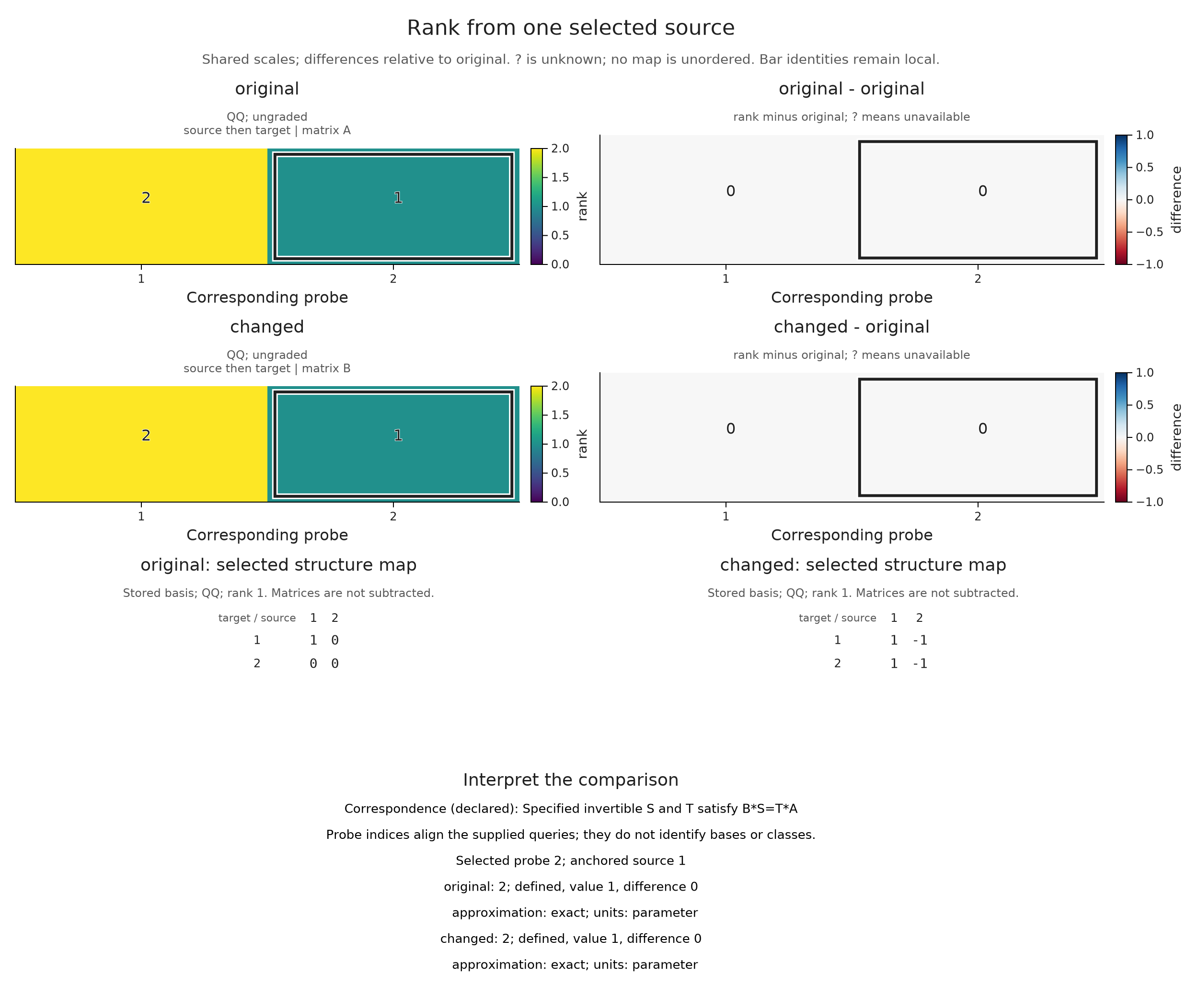
Change the finite description, preserve the parameters
Consider the module on the nonnegative plane with one copy of the field on $[0,2)\times[0,2)$ and zero elsewhere, with identity maps inside the square. One encoding uses the thresholds 0 and 2. Another inserts a cut at 1, subdividing the nonzero square without changing the module it represents. A vertex number in the first encoding need not name the same region in the second.
We therefore compare original parameter points. Each encoding map independently locates those points in its finite base. A point below zero lies outside both represented domains, so the display marks its value with ?. Inside the domain, a zero stalk remains an available answer.
coarse_poset = OP.Advanced.ProductOfChainsPoset((2,2))
fine_poset = OP.Advanced.ProductOfChainsPoset((3,3))
coarse_dims = [1,0,0,0]
fine_dims = [1,1,0,1,1,0,0,0,0]
coarse_module = OP.Advanced.PModule{OP.QQ}(coarse_poset, coarse_dims,
    Dict((a,b)=>ones(OP.QQ,coarse_dims[b],coarse_dims[a]) for (a,b) in OP.Advanced.cover_edges(coarse_poset)))
fine_module = OP.Advanced.PModule{OP.QQ}(fine_poset, fine_dims,
    Dict((a,b)=>ones(OP.QQ,fine_dims[b],fine_dims[a]) for (a,b) in OP.Advanced.cover_edges(fine_poset)))
coarse = OP.EncodingResult(coarse_poset, coarse_module,
    OP.Advanced.GridEncodingMap(coarse_poset, ([0,2],[0,2])))
fine = OP.EncodingResult(fine_poset, fine_module,
    OP.Advanced.GridEncodingMap(fine_poset, ([0,1,2],[0,1,2])));
points = [(-1,0), (0,0), (1//2,1//2), (3//2,3//2), (2,2)]
grids = OP.compare_visuals((
coarse=OP.ComparisonCase(coarse; filtration="coordinatewise sublevel", construction="cuts at 0 and 2", approximation="exact square"),
refined=OP.ComparisonCase(fine; filtration="coordinatewise sublevel", construction="additional cut at 1", approximation="exact subdivision"));
points, correspondence="Identical original coordinates in two encodings of the square")
OP.visualize(grids)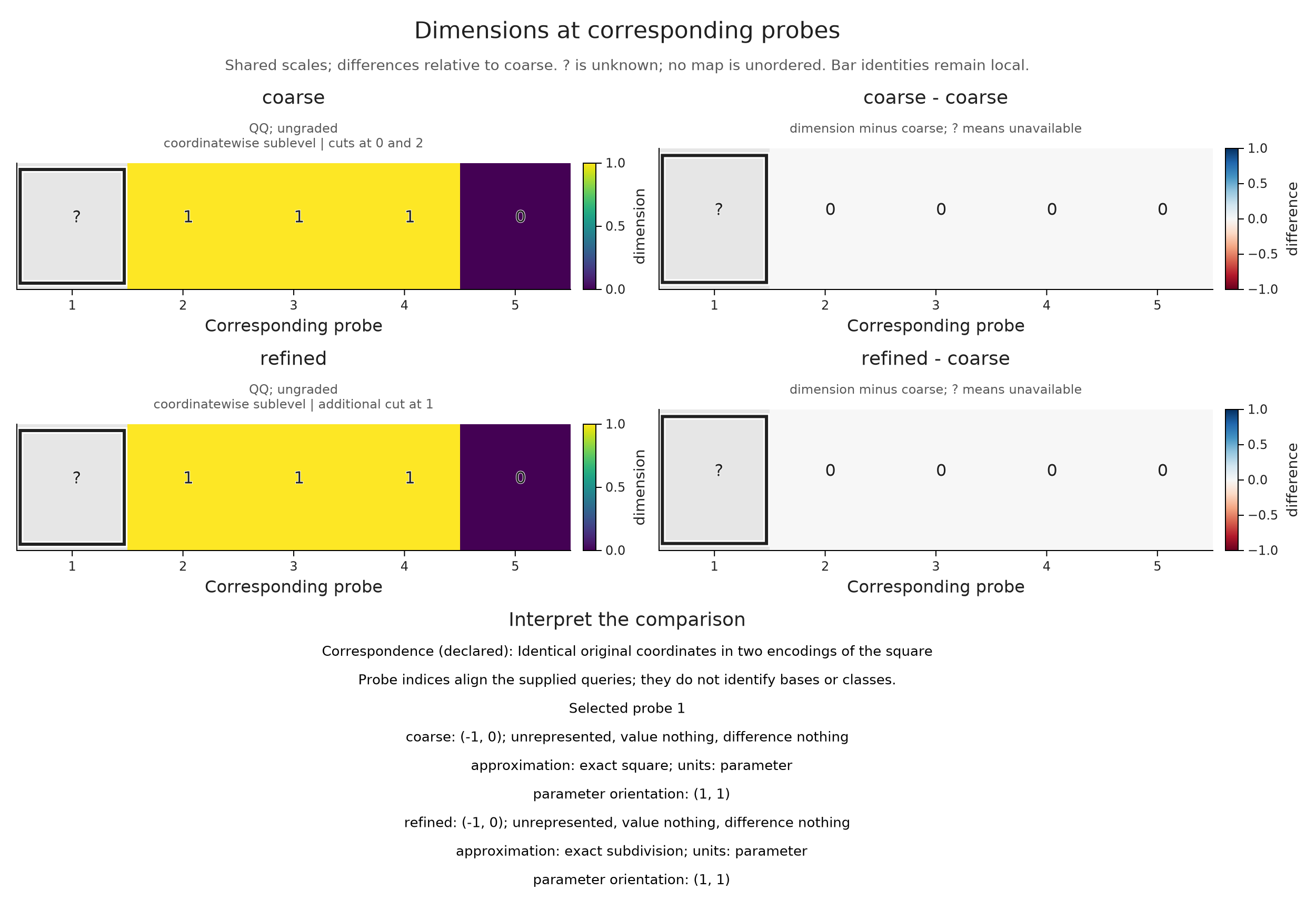
The two encodings agree on these queries. Their equality as descriptions of the module involves all spaces and maps, which we can investigate through an actual comparison map on a common refinement in refining and transporting encoded modules.
A rounding rule can change the query even when the encoding stays fixed. Rounding $(3/2,3/2)$ upward to $(2,2)$ crosses the square's excluded upper boundary, changing its dimension from one to zero. Separate point lists make that choice explicit below. The approximation description states the rule; a bound on the error in some other quantity would need a further argument.
rounded = OP.compare_visuals((
    exact=OP.ComparisonCase(coarse; filtration="coordinatewise sublevel", construction="original coordinates", approximation="exact query"),
    rounded=OP.ComparisonCase(coarse; filtration="coordinatewise sublevel", construction="ceil to integer grid", approximation="declared upward rounding"));
    points=(exact=[(0,0),(3//2,3//2),(2,2)], rounded=[(0,0),(2,2),(2,2)]),
    correspondence="Probe i uses the exact point on the left and its coordinatewise ceiling on the right")
OP.visualize(rounded)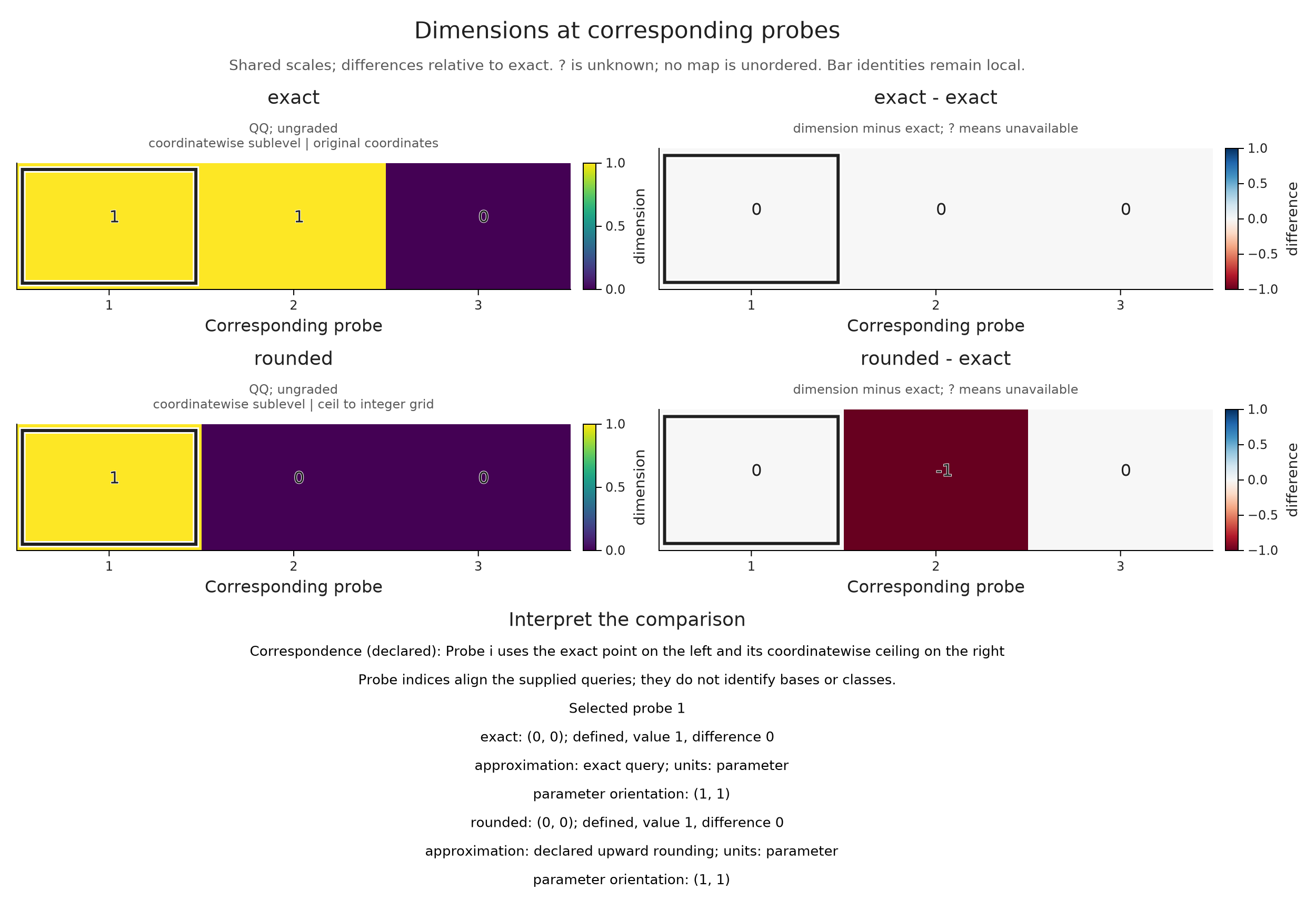
Compare barcodes in the same parameter units
For ordinary persistence results, the comparison can display intervals. Take an integral filtered chain complex with one generator in degree 0 at parameter 0 and one in degree 1 at parameter 1. Its differential multiplies by 2. Over $\mathbf F_2$, that differential vanishes, so the degree 0 class survives. Over $\mathbf F_3$, it becomes an isomorphism when the degree 1 generator appears, and the class dies at 1.
We use the same parameter queries and choose degree=0 for both results. The finite interval is $[0,1)$, so it has already disappeared at the query 1. The view distinguishes an essential interval, which continues indefinitely, from a finite interval clipped by a display window.
filtered_complex = OP.DataTypes.GradedComplex([[1],[2]], [sparse(reshape([2],1,1))], [(0,),(1,)])
diagram2 = OP.persistence_diagram(filtered_complex; field=F2)
diagram3 = OP.persistence_diagram(filtered_complex; field=F3)
bars = OP.compare_visuals((
    f2=OP.ComparisonCase(diagram2; degree=0, filtration="grades 0 then 1", construction="integral differential 2 modulo 2", approximation="exact"),
    f3=OP.ComparisonCase(diagram3; degree=0, filtration="grades 0 then 1", construction="integral differential 2 modulo 3", approximation="exact"));
    parameters=[0,1,2], window=(-1,3), correspondence="Same filtration parameter and homology degree")
OP.visualize(bars; view=:barcode, probe=2)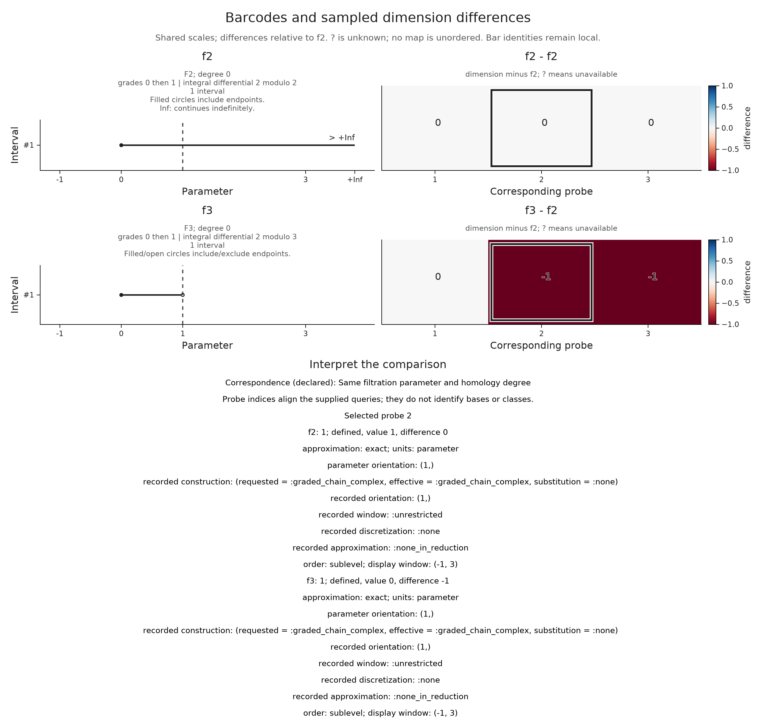
A row identifies a bar within its own result. Matching row numbers or colors between results does not assign one class to another. When that assignment is the question, the distance witness recipe computes and inspects a matching.
We can use a common parameter axis to compare homology degrees as well. In our complex over $\mathbf F_2$, the differential is zero, so the degree 1 generator creates a class at 1. At and after that parameter, degrees 0 and 1 both have dimension one. Their difference of zero describes dimensions of different spaces.
degrees = OP.compare_visuals((
    H0=OP.ComparisonCase(diagram2; degree=0, filtration="grades 0 then 1", construction="same filtered complex", approximation="exact"),
    H1=OP.ComparisonCase(diagram2; degree=1, filtration="grades 0 then 1", construction="same filtered complex", approximation="exact"));
    parameters=[0,1,2], correspondence="Same filtration parameters; distinct homology degrees")
OP.visualize(degrees; view=:barcode, probe=2)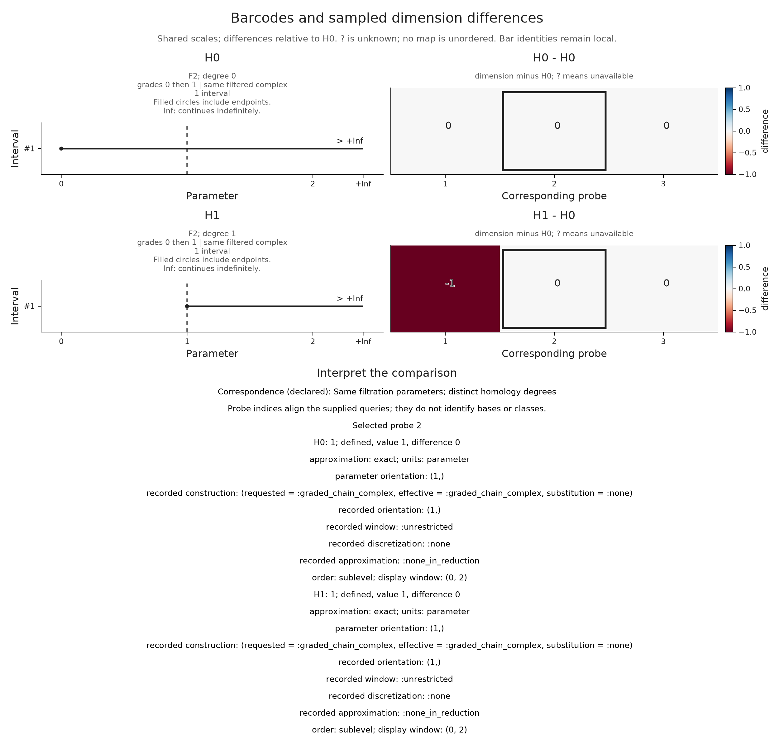
Keep numerical rank visible
With floating coefficients, the rank calculation depends on its tolerance. For $\operatorname{diag}(1,0.0008)$, an absolute tolerance of 0.001 discards the smaller direction, while the corresponding rational matrix has exact rank two. We specify both the absolute and relative tolerances so this decision can be read beside the result.
The view repeats its numerical rank check at half and double the declared tolerances. Here halving the tolerance restores the second direction and reveals sensitivity to that choice. Agreement among those three calculations would still say only that these particular tolerance changes left the answer unchanged.
real_field = OP.CoreModules.RealField(Float64; atol=0.001, rtol=0.0)
numerical = OP.Advanced.PModule{Float64}(P, [2,2], Dict((1,2)=>[1.0 0; 0 0.0008]); field=real_field)
rational = OP.Advanced.PModule{OP.QQ}(P, [2,2], Dict((1,2)=>OP.QQ[1 0; 0 8//10000]))
tolerances = OP.compare_visuals((
    numerical=OP.ComparisonCase(numerical; filtration="source then target", construction="Float64 diagonal", approximation="rank with specified tolerance"),
    rational=OP.ComparisonCase(rational; filtration="source then target", construction="rational diagonal", approximation="exact reference"));
    vertices=(numerical=[1,2], rational=[1,2]), correspondence="Declared rational matrix and its floating-point representation")
OP.visualize(tolerances; view=:rank, probe=2)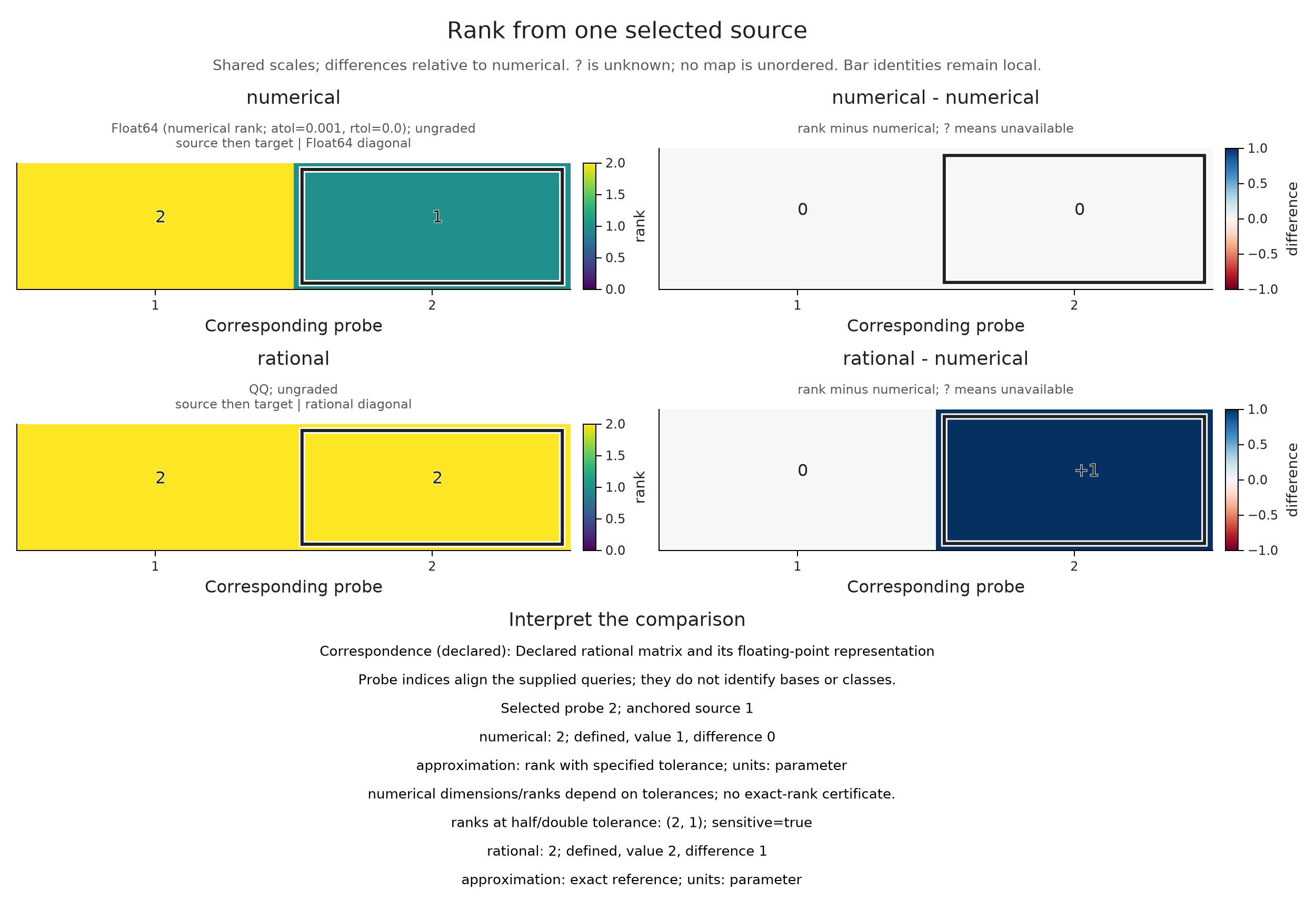
Explore linked selections
With WGLMakie loaded, the same comparison can be opened in a live inspector while Julia is running:
import WGLMakie
session = OP.inspection_session(fields)
OP.visualize(session; backend=:wglmakie)
Clicking a value or difference strip selects a query. The Anchored ranks option asks for maps from the source chosen in its field; Baseline case chooses which case to subtract. Inspect selected matrices displays the corresponding maps in their stored bases. When two vertices are incomparable, the readout says “no map,” since the poset module prescribes no map for that pair.
The inspector computes only the requested source row of ranks, reusing it when the target or baseline changes. For a lazy encoding, the first nontrivial map query also constructs the finite module. Hover reads retained values. Keep the compared inputs unchanged during use and prepare a new comparison after editing them. The session guide explains supported display paths, linked views and closing; the final static snapshot remains available after a session closes.
Compare samples through named features
So far, a position in a comparison has represented one query inside a result. For a collection, let each row represent an entire sample and each column a named feature of it. We need to retain these row identities as we move from the feature table to another view.
Consider three interval modules: A lives on $[0,2)$, B on $[0,3)$, and C on $[2,4)$. Record each interval's lifetime and its dimension at parameter 1. The feature rows are $(2,1)$, $(3,1)$ and $(2,0)$. A and C have the same lifetime, but only A is present at the selected parameter.
Featurizers.FeatureSet stores a row for each sample and a column for each feature. It is also the container returned by batch featurization. Here we supply the values calculated above so their meanings stay visible. Their units differ, and we apply no normalization.
bars = [[(0.,2.)], [(0.,3.)], [(2.,4.)]]
features = OP.Featurizers.FeatureSet(
    [2. 1.; 3. 1.; 2. 0.], [:lifetime, :dimension_at_one], ["A", "B", "C"],
    (;interval_convention="[birth, death)", parameter=1, normalization="none"))
definitions = ["Death minus birth of the single finite interval",
               "Dimension of the interval module at parameter 1"]
collection = OP.visual_collection(features; definitions, degree=0, field="F2")
OP.visualize(collection)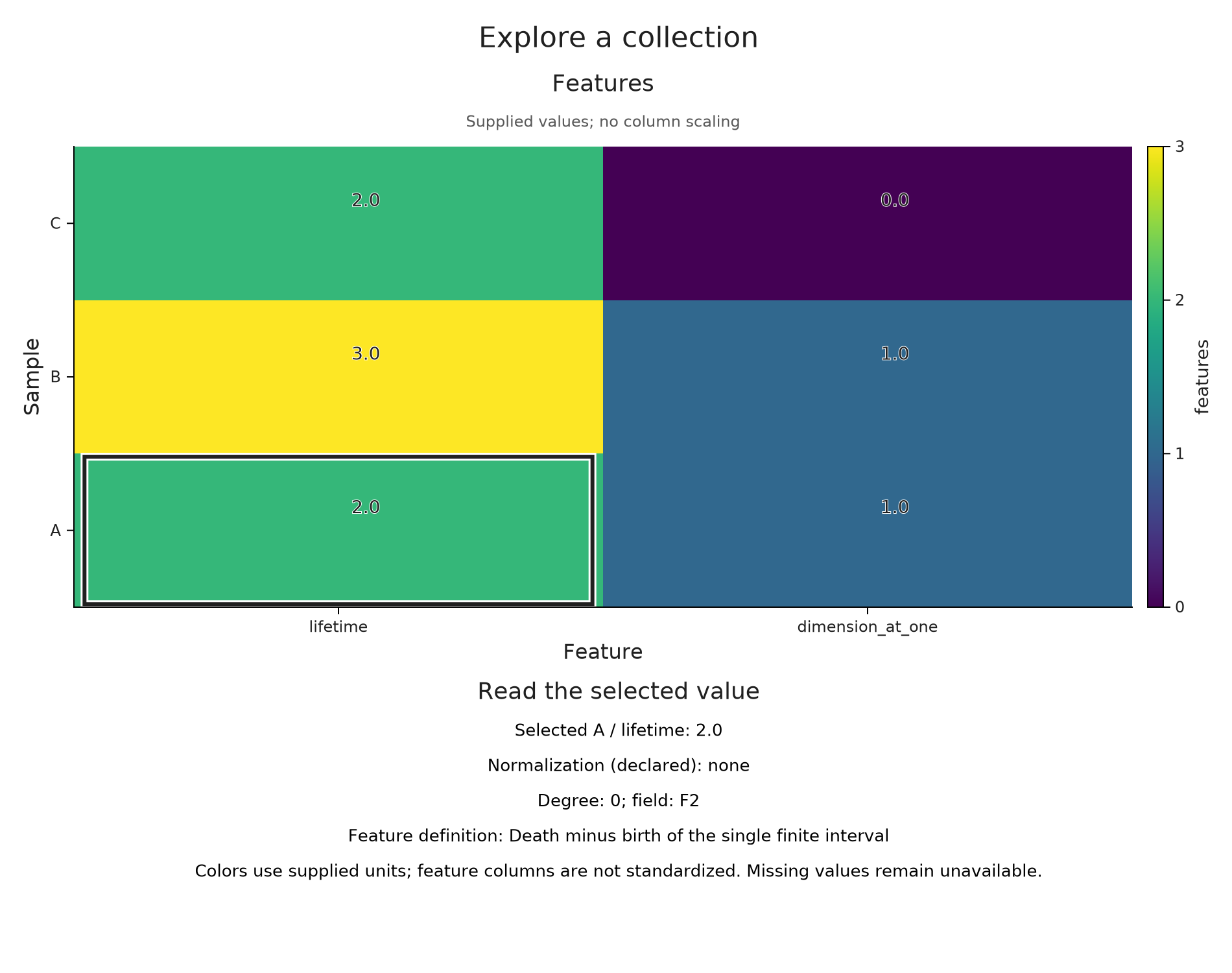
The labels retain the sample IDs and feature names. The color scale covers the supplied numbers: a color for a lifetime of two and a color for a dimension of two would indicate equal numerical values with different meanings. If you standardize the columns elsewhere, record that transformation in normalization, including how its parameters were fitted.
Compare the intervals by distance
A distance between the original intervals asks a further question. Their bottleneck distances are $d(A,B)=1$, $d(A,C)=1$, and $d(B,C)=3/2$. In the last two comparisons, the optimum matches each interval to the diagonal, paying half its lifetime. For example, directly matching B to C costs two, whereas sending both to the diagonal costs $\max(3/2,1)=3/2$.
We supply this small table explicitly; preparing a collection does not compute all pairs. We also retain each sample's barcode, allowing a selection to return from a table entry to the intervals being compared. A point cloud, graph or image could supply a further source view, but our abstract interval modules have no such data.
sample_views = [(;object=bar, invariant=OP.Advanced.visual_spec(bar),
                  metadata=(interval=only(bar), convention="[birth, death)")) for bar in bars]
distances = [0. 1. 1.; 1. 0. 1.5; 1. 1.5 0.]
witness_AB = OP.bottleneck_matching(bars[1], bars[2])
collection = OP.visual_collection(features; definitions, distances,
    distance_semantics="Bottleneck distance, L-infinity ground cost, diagonal allowed",
    degree=0, field="F2", samples=sample_views,
    witnesses=Dict(("A", "B")=>witness_AB))
OP.visualize(collection; view=:distances, sample="B", target="C")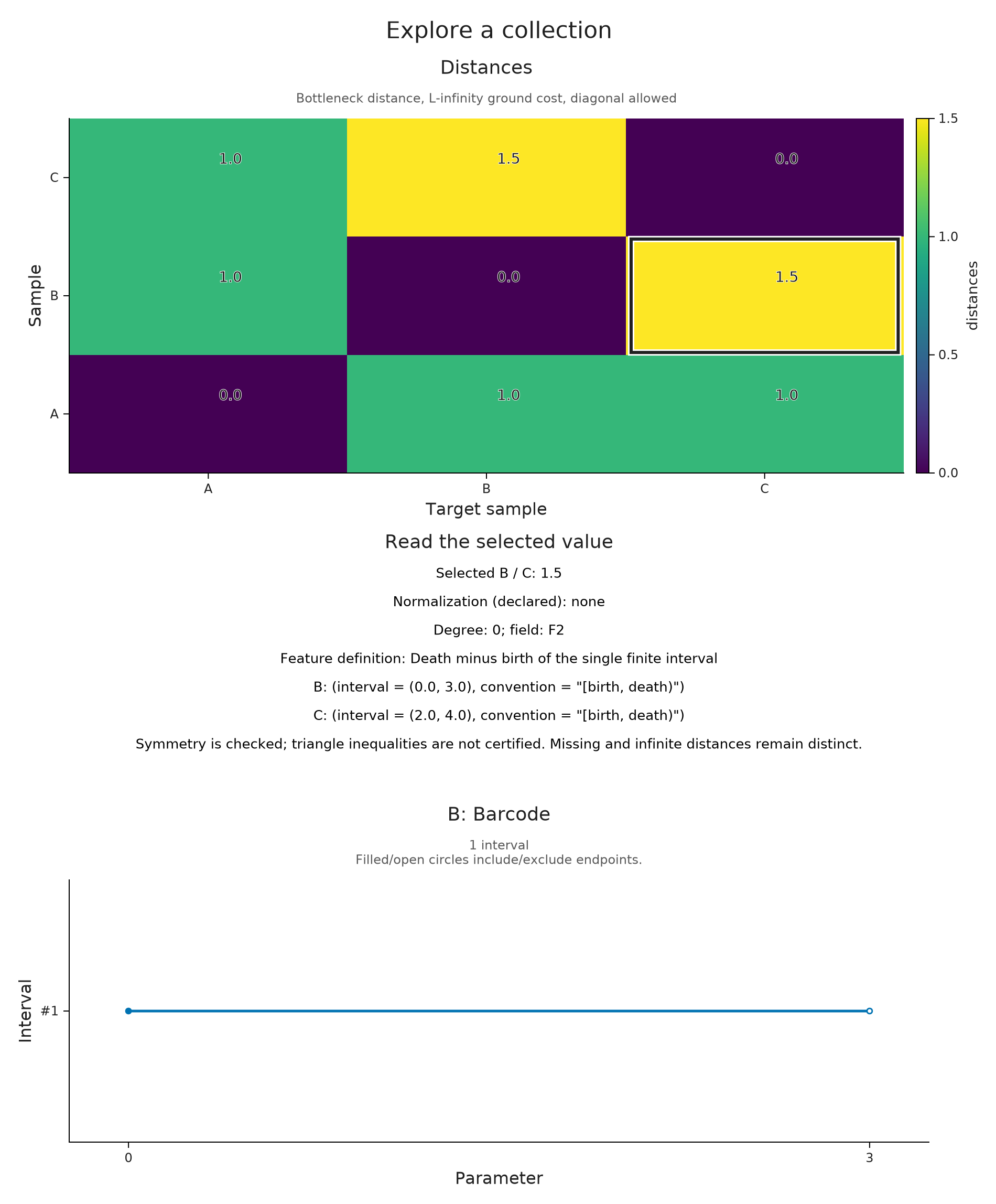
For a distance table, the constructor checks its shape, signs and symmetry. The triangle inequality remains a mathematical property to establish for the supplied distances. An unavailable pair is recorded as missing, and an infinite distance as Inf, preserving both distinctions from zero.
A kernel table records similarities. In the common positive semidefinite case, every quadratic form $c^TKc$ is nonnegative, but the viewer does not certify this condition. Pass such a table as kernel and describe its meaning with kernel_semantics; its diagonal generally differs from zero, and individual entries may be negative.
Our example uses dot products of the two feature coordinates, so $K=XX^T$, where $X$ is the feature matrix. This construction is positive semidefinite because $c^TKc=\lVert X^Tc\rVert^2$. Its values depend on the units and scaling of those features.
similarities = [5. 7. 4.; 7. 10. 6.; 4. 6. 4.]
kernel_collection = OP.visual_collection(features; definitions, kernel=similarities,
    kernel_semantics="Dot product of lifetime and dimension-at-one coordinates",
    degree=0, field="F2")
OP.visualize(kernel_collection; view=:kernel, sample="B", target="B")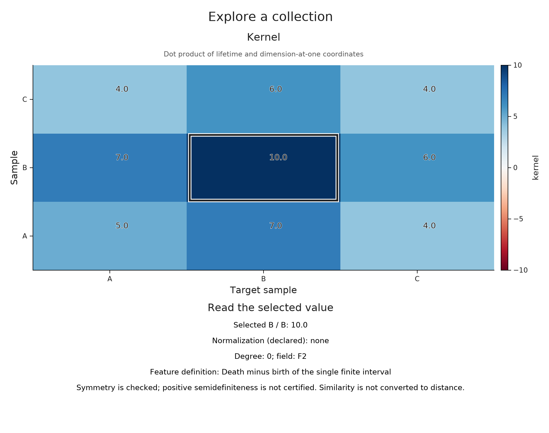
Place samples in plotting coordinates
An embedding assigns plotting coordinates to each sample, often through a transformation supplied by another tool. visual_collection accepts those coordinates together with the method, settings and seed used to obtain them. Here the two feature columns already provide coordinates, so no fitted transformation is needed.
B and C are $\sqrt{2}$ apart in this plot, while their bottleneck distance is $3/2$. Both values have a clear meaning: one measures Euclidean separation of the chosen feature coordinates, and the other compares the intervals. Reading the table beside the plot keeps that distinction visible.
The viewer below keeps the three pairs A–B, A–C and B–C available. Its selected matrix cell, highlighted feature coordinates and two barcodes follow the same pair. Compare A–B with A–C: both bottleneck distances are one, although the intervals achieve those distances through different assignments. The parameter window stays fixed as the selected pair changes.
embedded = OP.visual_collection(features; definitions, distances,
    distance_semantics="Bottleneck distance, L-infinity ground cost, diagonal allowed",
    degree=0, field="F2", samples=sample_views,
    embedding=(coordinates=OP.Featurizers.feature_matrix(features),
               method="Lifetime and dimension at 1", settings=(axes=(:lifetime,:dimension_at_one),), seed=nothing))
OP.visualize(embedded; view=:distances, sample="B", target="C")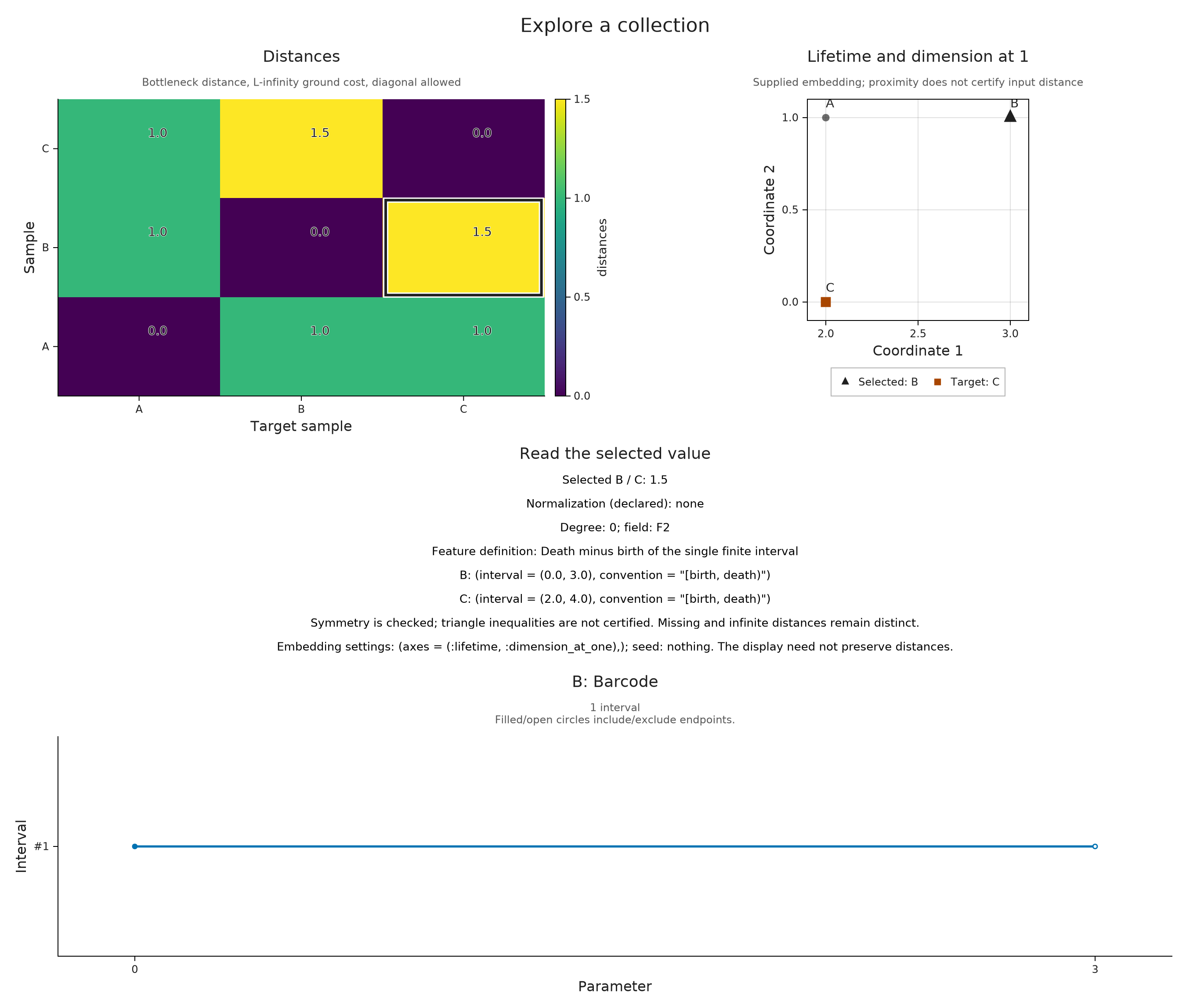
Explore the three interval pairs
Open the selected pair
The collection inspector links its table, plotting coordinates and retained sample views through the same sample IDs. The sample and target choices identify a pair consistently in each panel. Feature selection exposes its definition, and hover reads prepared values without recomputing an invariant or a distance.
When a matching witness has been supplied, collection_matching opens it in the matching explorer. Its assignment distinguishes source from target, so it belongs to an ordered pair. The witness must have the mathematical meaning you intend; storing it beside an arbitrary table does not certify that table's values.
collection_session = OP.inspection_session(collection; view=:distances)
pair_session = OP.collection_matching(collection_session)
@assert OP.Advanced.inspection_snapshot(pair_session).metadata.matching_records !== nothing
OP.visualize(OP.Advanced.inspection_snapshot(pair_session))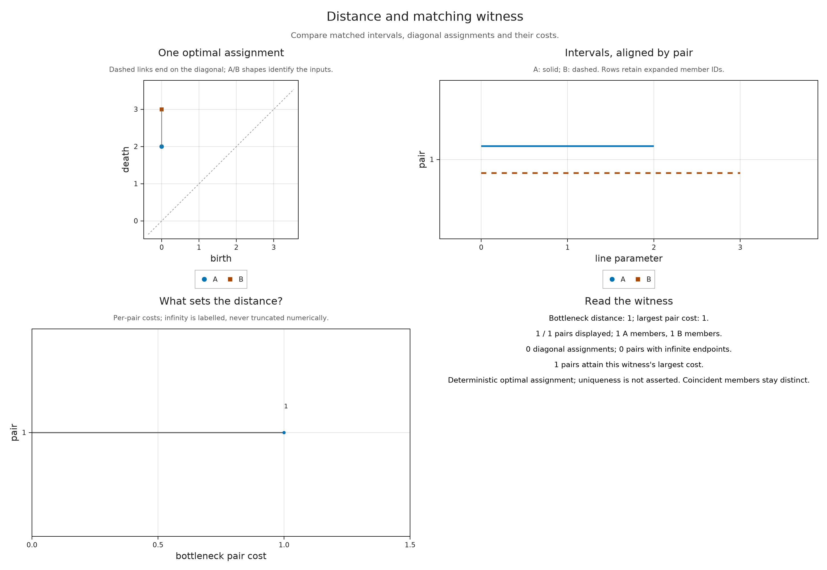
With WGLMakie loaded, OP.visualize(collection_session; backend=:wglmakie) opens the live controls. Clicking a matrix cell selects its row and column, while clicking a plotted sample selects its ID. Open supplied matching opens the retained witness for that ordered pair. Changing the parent selection closes that embedded pair view; separate sessions created in Julia remain independently usable.
For a pair without a retained witness, compute=true requests a calculation. Below we ask only for B against C, using their retained interval objects, and check the predicted distance $3/2$. Ordinary PersistenceDiagram inputs additionally require dim; encoded pairs require their finite window options. The API reference describes those contracts and budgets. Computing one pair leaves the supplied table unchanged.
OP.Advanced.select_inspection!(collection_session; sample="B", target="C")
pair_BC = OP.collection_matching(collection_session; compute=true)
selected_distance = OP.Advanced.inspection_summary(pair_BC).distance
@assert selected_distance == 1.5
selected_distance1.5OP.Advanced.close_inspection!(pair_BC)
OP.Advanced.close_inspection!(pair_session)
OP.Advanced.close_inspection!(collection_session);Optional: prepare a figure for sharing
The default views already include the context needed to interpret the numbers. Styling and export are independent of those calculations. This grayscale export uses the same prepared rank answer.
sharing_style = OP.VisualStyle(palette=:grayscale)
OP.visualize(rank_view; style=sharing_style)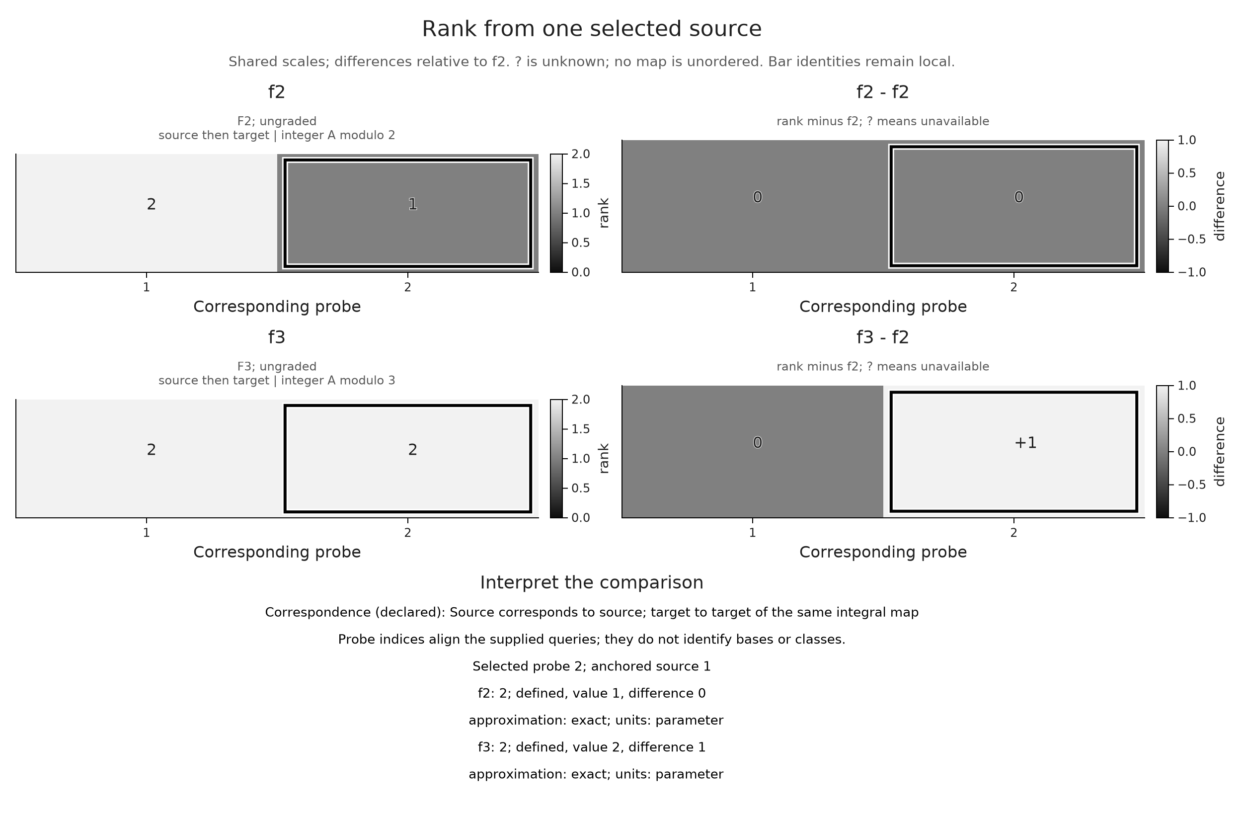
export_directory = mktempdir()
OP.save_visual(joinpath(export_directory, "field-ranks.svg"), rank_view; style=sharing_style);
The following exports retain the choices used in the prepared viewers. We select the plot panels that answer each comparison and keep their common scales. The original comparison objects still retain their full context for inspection in Julia.
field_choices = (
    (name="Source identity; subtract F2", probe=1, baseline=:f2),
    (name="Target map; subtract F2", probe=2, baseline=:f2),
    (name="Target map; subtract F3", probe=2, baseline=:f3))
field_views = Pair{Symbol,Any}[]
for choice in field_choices
    selected_comparison = OP.Advanced.visual_spec(fields; view=:rank, source=1,
        probe=choice.probe, baseline=choice.baseline, matrix=true)
    @assert [v.value for v in selected_comparison.metadata.values.f2] == [2,1]
    @assert [v.value for v in selected_comparison.metadata.values.f3] == [2,2]
    @assert selected_comparison.metadata.colorrange == (0.,2.)
    @assert selected_comparison.metadata.difference_range == (-1.,1.)
    expected_difference = choice.baseline == :f2 ? 1 : -1
    other_case = choice.baseline == :f2 ? :f3 : :f2
    @assert selected_comparison.metadata.differences[other_case][2].value == expected_difference
    figure = OP.compose_visuals((
        ranks_f2=OP.visual_panel(selected_comparison; panel=1),
        difference_f2=OP.visual_panel(selected_comparison; panel=2),
        ranks_f3=OP.visual_panel(selected_comparison; panel=3),
        difference_f3=OP.visual_panel(selected_comparison; panel=4),
        matrix_f2=OP.visual_panel(selected_comparison; panel=5),
        matrix_f3=OP.visual_panel(selected_comparison; panel=6));
        columns=2, title=choice.name,
        subtitle="Query 1 is the source; query 2 is the target. All maps start at the source.")
    push!(field_views, Symbol(choice.name) => figure)
end
field_viewer_path = joinpath("tamerop_outputs", "comparisons", "fields.html")
mkpath(dirname(field_viewer_path))
OP.save_visual_session(field_viewer_path,
    (; field_views...); selected=Symbol("Target map; subtract F2"),
    title="Compare ranks over two coefficient fields",
    caption="The integral matrix has rows (1,1) and (1,-1). Reduction modulo 2 gives rank 1; reduction modulo 3 gives rank 2. The difference panels subtract the chosen field's ranks. Changing that baseline changes differences without changing either map.",
    style=OP.VisualStyle(fontsize=18), size=(1100,1100));
pair_views = Pair{Symbol,Any}[]
for (i,j,expected_distance) in ((1,2,1.), (1,3,1.), (2,3,1.5))
    sample, target = OP.Featurizers.sample_ids(features)[i], OP.Featurizers.sample_ids(features)[j]
    selected_pair = OP.Advanced.visual_spec(embedded; view=:distances, sample, target)
    @assert selected_pair.metadata.selected.value == expected_distance
    @assert selected_pair.metadata.selected.sample == sample
    @assert selected_pair.metadata.selected.target == target
    figure = OP.compose_visuals((
        distances=OP.visual_panel(selected_pair; panel=:collection_matrix),
        coordinates=OP.visual_panel(selected_pair; panel=:collection_embedding),
        sample=OP.visual_panel(bars[i]; kind=:barcode, window=(0,4), title="Sample $sample"),
        target=OP.visual_panel(bars[j]; kind=:barcode, window=(0,4), title="Target $target"));
        columns=2, title="$sample and $target: bottleneck distance $expected_distance",
        subtitle="Feature coordinates: lifetime horizontally; dimension at parameter 1 vertically.")
    push!(pair_views, Symbol("$sample and $target") => figure)
end
pair_viewer_path = joinpath("tamerop_outputs", "comparisons", "pairs.html")
mkpath(dirname(pair_viewer_path))
OP.save_visual_session(pair_viewer_path,
    (; pair_views...); selected=Symbol("B and C"),
    title="Follow a pair from its distance to its intervals",
    caption="The table gives bottleneck distances with the L-infinity cost and diagonal matching allowed. Feature coordinates are supplied without normalization and need not preserve these distances. The barcodes use the same parameter window and half-open intervals in degree zero over F₂.",
    style=OP.VisualStyle(fontsize=18), size=(1180,1000));
The examples let us trace each comparison to its question: a field changes a map's rank, a basis changes its matrix, and a rounding rule changes the parameter being queried. In a collection, the feature definitions and sample IDs provide the same continuity from a number back to its interval or matching witness. For actual maps between finite descriptions, continue to refining and transporting encoded modules. To assemble these views into a larger figure, see composing mathematical figures.