Exploring slices, intervals and signed contributions
Download the executed notebook · Build and environment record
A finite encoding retains vector spaces and the maps between them, so we can ask how a class continues along a line or how many independent vectors survive from one parameter to another. These questions lead to different summaries of the same module. We will follow a small example through a slice barcode and two signed sums, working out why a negative coefficient is needed even though every rank and dimension is nonnegative.
Use Julia with TamerOp and CairoMakie, and recall how the spaces and maps of a finite encoding describe a module. Our input is a supplied finite diagram over the rational numbers. After the worked queries, optional sections explain how to move a slice, distinguish an endpoint from a viewing boundary, and inspect repeated intervals.
using TamerOp, CairoMakie
const A = TamerOp.Advanced
const F = TamerOp.FiniteFringe
const E = TamerOp.EncodingCore
const Mds = TamerOp.Modules
const S = TamerOp.SignedMeasures
TamerOp.SignedMeasuresOne module, several questions
Use the grid with coordinates 0, 2 and 5 on each axis. Every label carries a one dimensional space except the last label, at (5,5), whose space is zero. Maps between nonzero spaces are identities. Extending each label's value from its grid coordinate up to the next coordinate gives a horizontal strip and a vertical strip that overlap near the origin. Following the diagonal eventually leaves both strips, so its class must die.
The classifier assigns a parameter to the label at the greatest grid coordinate below it in each direction. We use zero spaces below the first coordinates and constant values beyond the last ones. Thus the regions include their lower edges and exclude their upper edges; the two strips continue indefinitely in their long directions. These conventions determine the endpoints that appear in the figures.
coordinates = [0, 2, 5]
P = F.ProductOfChainsPoset((3, 3))
classifier = E.GridEncodingMap(P, (coordinates, coordinates))
field = TamerOp.CoreModules.QQField()
K = Rational{BigInt}
stalk_dimensions = [x <= 2 || y <= 2 ? 1 : 0 for y in coordinates for x in coordinates]
maps = Dict((a,b) => fill(one(K), stalk_dimensions[b], stalk_dimensions[a])
            for (a,b) in F.cover_edges(P))
module_ = Mds.PModule{K}(P, stalk_dimensions, maps; field)
encoding = TamerOp.Results.EncodingResult(P, module_, classifier)
TamerOp.describe(encoding)
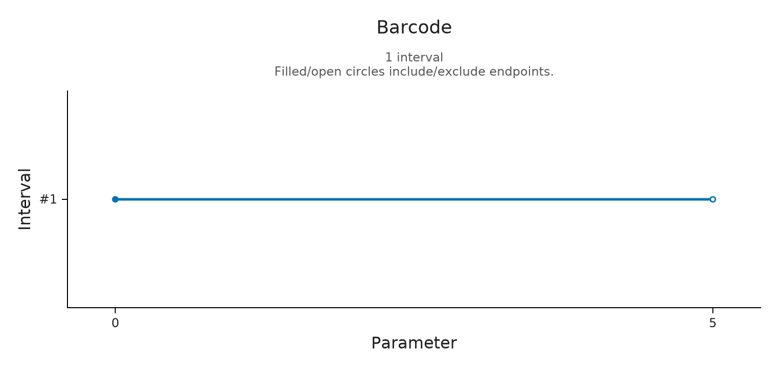
(kind = :encoding_result, poset_type = TamerOp.FiniteFringe.ProductOfChainsPoset{2}, module_type = TamerOp.Modules.PModule{Rational{BigInt}, TamerOp.CoreModules.CoeffFields.QQField, Matrix{Rational{BigInt}}, TamerOp.FiniteFringe.ProductOfChainsPoset{2}}, encoding_map_type = TamerOp.EncodingCore.GridEncodingMap{2, Int64, TamerOp.FiniteFringe.ProductOfChainsPoset{2}}, compiled = false, backend = :auto, has_cohomology = false, has_presentation = false, module_dims = [1, 1, 1, 1, 1, 1, 1, 1, 0], materialized = true, provenance = (category = :finite_poset_representations, base_poset = ProductOfChainsPoset(axes=(3, 3), orientation=(1, 1), nvertices=9), field = TamerOp.CoreModules.CoeffFields.QQField(), degree = nothing, degree_convention = :not_applicable, encoding = (map_type = TamerOp.EncodingCore.GridEncodingMap{2, Int64, TamerOp.FiniteFringe.ProductOfChainsPoset{2}}, backend = :auto), window = :not_recorded, orientation = :not_recorded, construction = (requested = :not_recorded, effective = :not_recorded, substitution = :not_recorded), discretization = :not_recorded, approximation = :not_recorded, backend = (requested = :not_recorded, effective = :auto), ambient_identification = :not_asserted))On the diagonal, labels 1, 5 and 9 occur at parameter values 0, 2 and 5. The first two spaces are connected by the identity and the last is zero, giving one interval [0,5). Our explicit chain contains every change of the module along this diagonal.
diagonal = slice_barcode(module_, [1, 5, 9]; values=[0, 2, 5])
@assert diagonal == Dict((0, 5) => 1)
visualize(diagonal; kind=:barcode)
Why the rank description needs a negative term
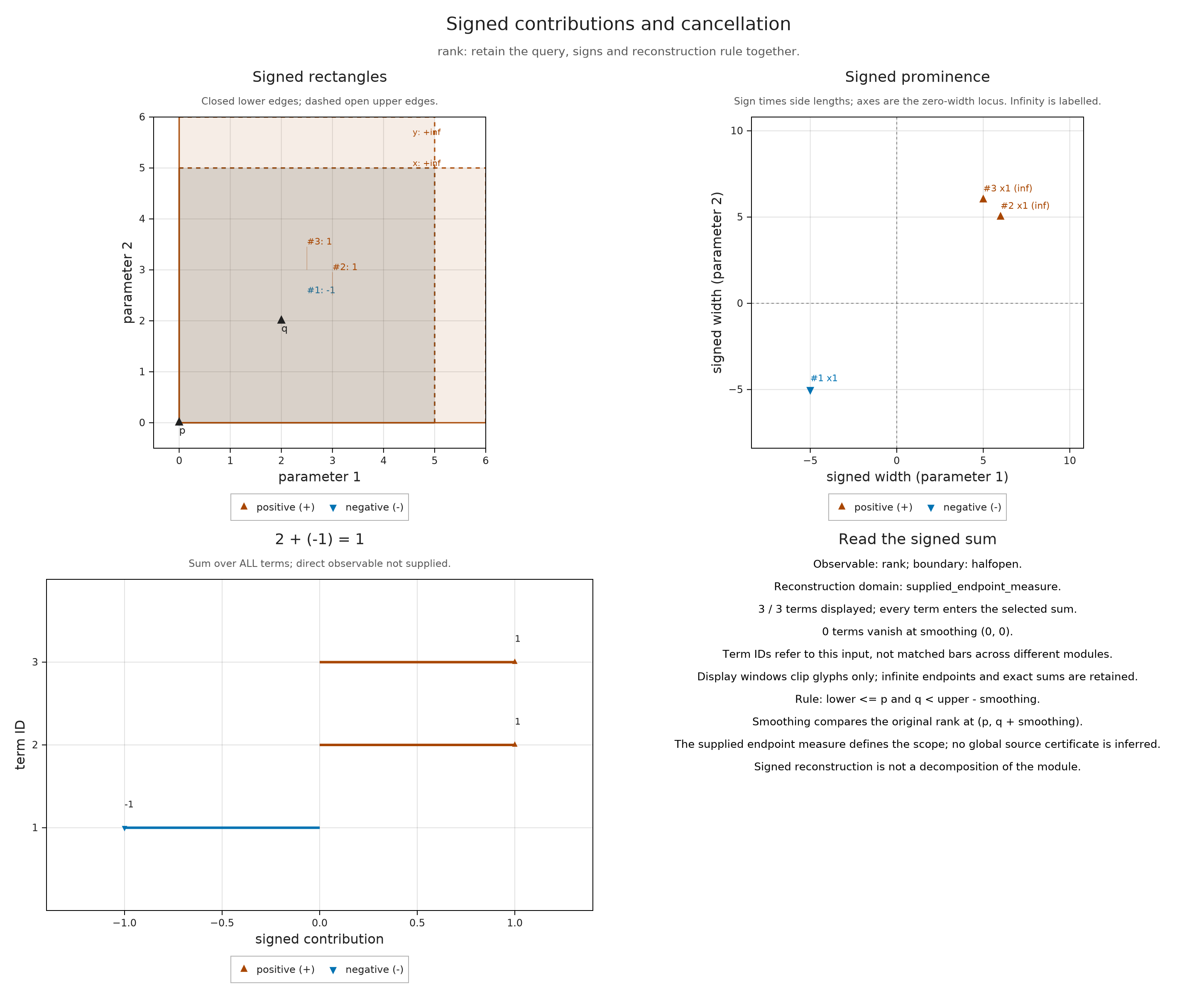
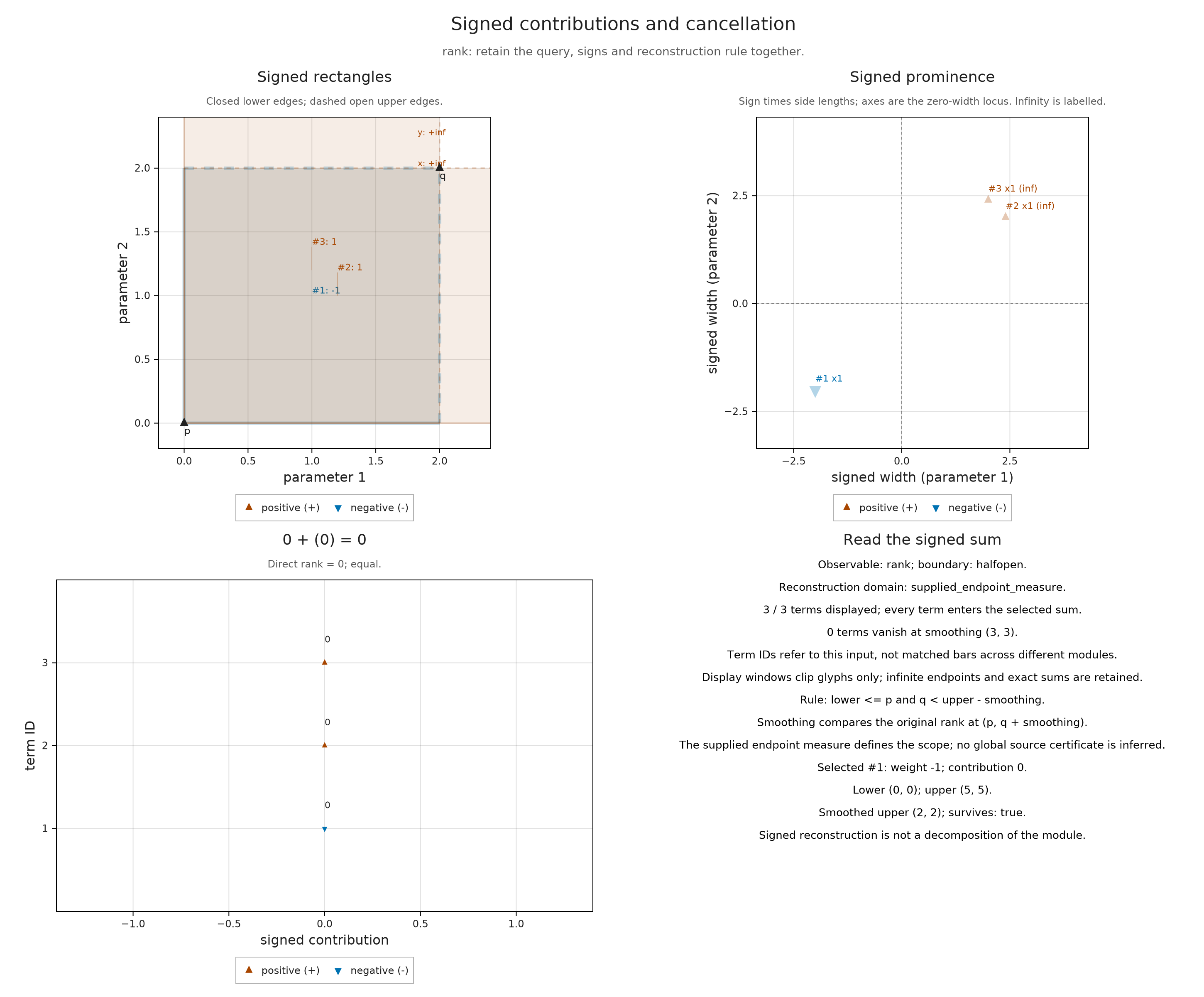
The rank from a parameter $p$ to a comparable parameter $q$ is the dimension of the image of their structure map. rank_signed_measure records this function as a finite sum of rectangle contributions with integer coefficients. Each term stores a two dimensional birth and death, hence four endpoint coordinates. It contributes when both $p$ and $q$ lie in its rectangle, with the endpoint conventions shown in the figure.
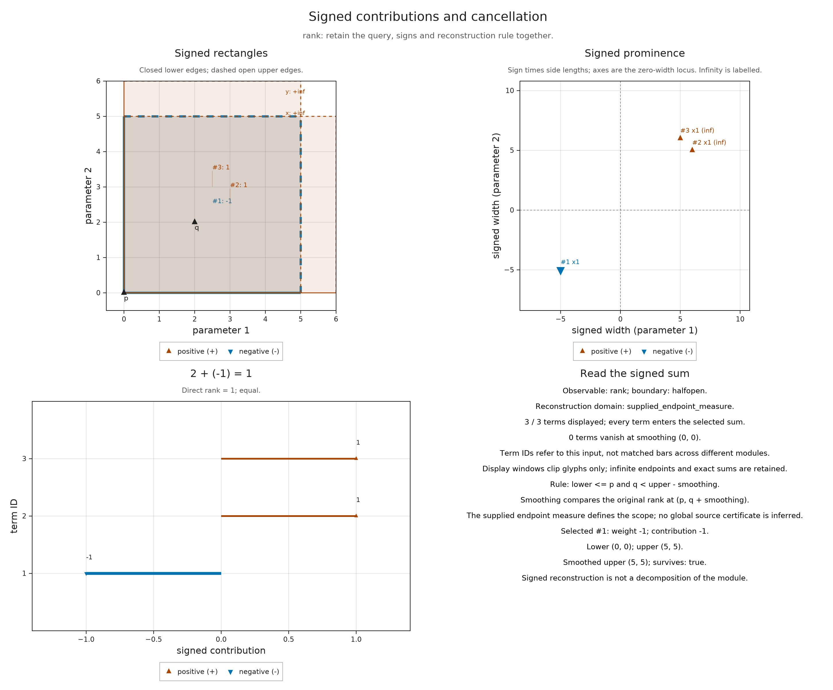
For the map from (0,0) to (2,2), both strips contain both points. Counting each strip once would give two, although our map is the identity on one line. Subtracting their overlap leaves the required rank one. In the adjacent prominence panel, the side lengths of positive terms lie in the positive quadrant and those of negative terms in the negative quadrant. Term labels keep the correspondence with the rectangles. A labelled infinite side has a finite drawing position so that it fits on the page; it still represents an unbounded rectangle.
rank_measure = rank_signed_measure(encoding; threads=false)
visualize(rank_measure; query=(p=(0,0), q=(2,2)))
We can check this reconstruction against the map we started with. The function below locates the finite labels of $p$ and $q$, then computes the rank of the actual matrix between them. It uses no signed coefficients, so agreement compares two descriptions of this query. Selecting the negative term highlights the overlap, its side lengths and the correction it contributes.
direct_rank = (p,q) -> TamerOp.Invariants.rank_map(module_,
    E.locate(classifier, collect(p)), E.locate(classifier, collect(q)))
negative_term = findfirst(<(0), S.weights(rank_measure))
signed_view = A.visual_spec(rank_measure; query=(p=(0,0), q=(2,2)),
    direct=direct_rank, term=negative_term)
@assert signed_view.metadata.agreement == :equal
@assert signed_view.metadata.reconstructed == 1
visualize(signed_view)
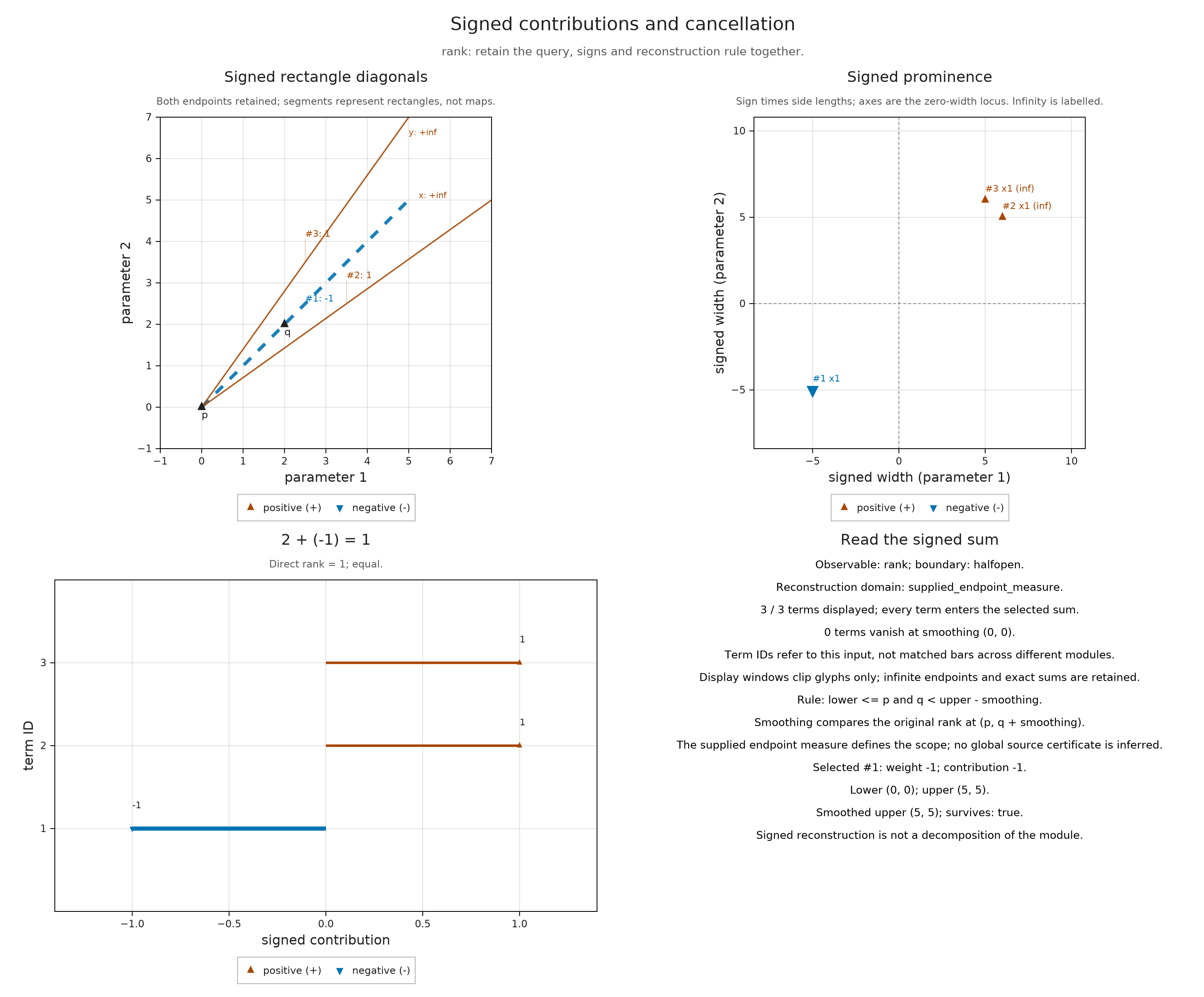
A diagonal from birth to death gives a less crowded view of each rectangle. These drawn segments represent endpoint pairs, not structure maps. Positive and negative terms have different marker shapes as well as colors. The chosen window clips the drawing while leaving infinite endpoints and the reconstructed sum unchanged.
visualize(rank_measure; kind=:signed_diagonals, query=(p=(0,0), q=(2,2)),
    direct=direct_rank, term=negative_term, window=((-1,-1),(7,7)))
Follow a class farther by smoothing
Let $\varepsilon$ be a vector with nonnegative coordinates. The smoothed module at $p$ is the image of the map from $M_p$ to $M_{p+\varepsilon}$, so it retains the classes that survive that additional displacement. Its rank from $p$ to $q$ equals the original rank from $p$ to $q+\varepsilon$. In the rectangle description, this moves each upper endpoint by $-\varepsilon$ and removes rectangles that become empty. This is the smoothing defined by Botnan, Oppermann and Oudot, §6.2; it is an operation on the module, with no averaging of plotted pixel values.
At $\varepsilon=(3,3)$, our query tests the original map from (0,0) to (5,5). The target space is zero, so the smoothed rank must be zero. The upper edges are excluded: arriving exactly at (5,5) is already enough to lose the class.
smoothed_view = A.visual_spec(rank_measure; query=(p=(0,0), q=(2,2)),
    smoothing=(3,3), direct=direct_rank, term=negative_term)
@assert smoothed_view.metadata.agreement == :equal
@assert smoothed_view.metadata.reconstructed == 0
visualize(smoothed_view)
Dimensions use a different signed sum
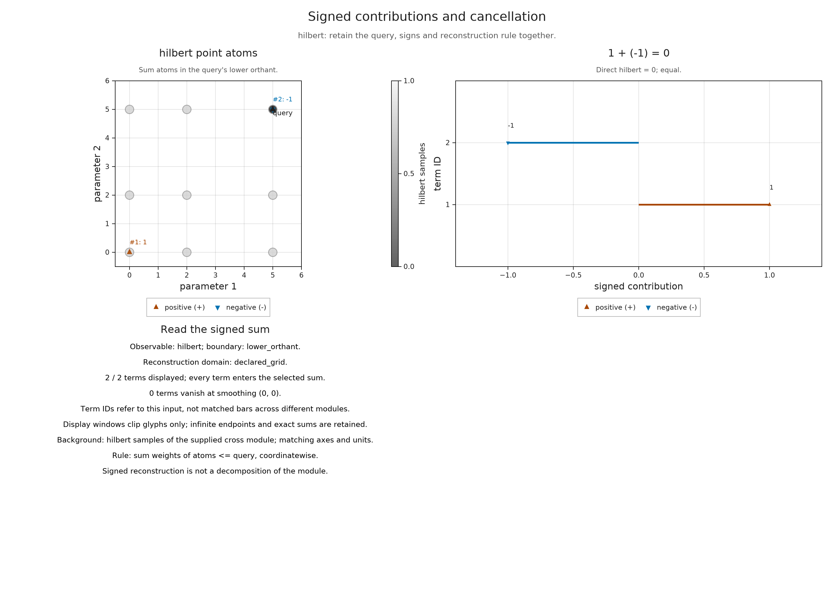
The Hilbert function gives the dimension of the module at each parameter. It has one parameter input, whereas the rank function has a source and target. Its signed representation therefore uses point terms: a term contributes when its point lies coordinatewise below the query. At (5,5), the birth contributes +1 and a correction contributes −1, recovering the zero dimensional space there.
The colored background samples below come from this same Hilbert function. They are individual sample points, with no interpolation between them. The background matrix has rows for $y$ and columns for $x$, so we transpose the array whose first index was $x$ before drawing it.
hilbert = [restricted_hilbert(module_, classifier, [x,y]) for x in coordinates, y in coordinates]
atoms = S.point_signed_measure(hilbert, (coordinates, coordinates))
background = (axes=(coordinates, coordinates), values=permutedims(hilbert),
    observable=:hilbert, source="the supplied cross module", units=("parameter 1", "parameter 2"))
visualize(atoms; kind=:signed_cancellation, observable=:hilbert, query=(5,5),
    direct=p -> restricted_hilbert(module_, classifier, collect(p)), background)
A declared family of finite regions
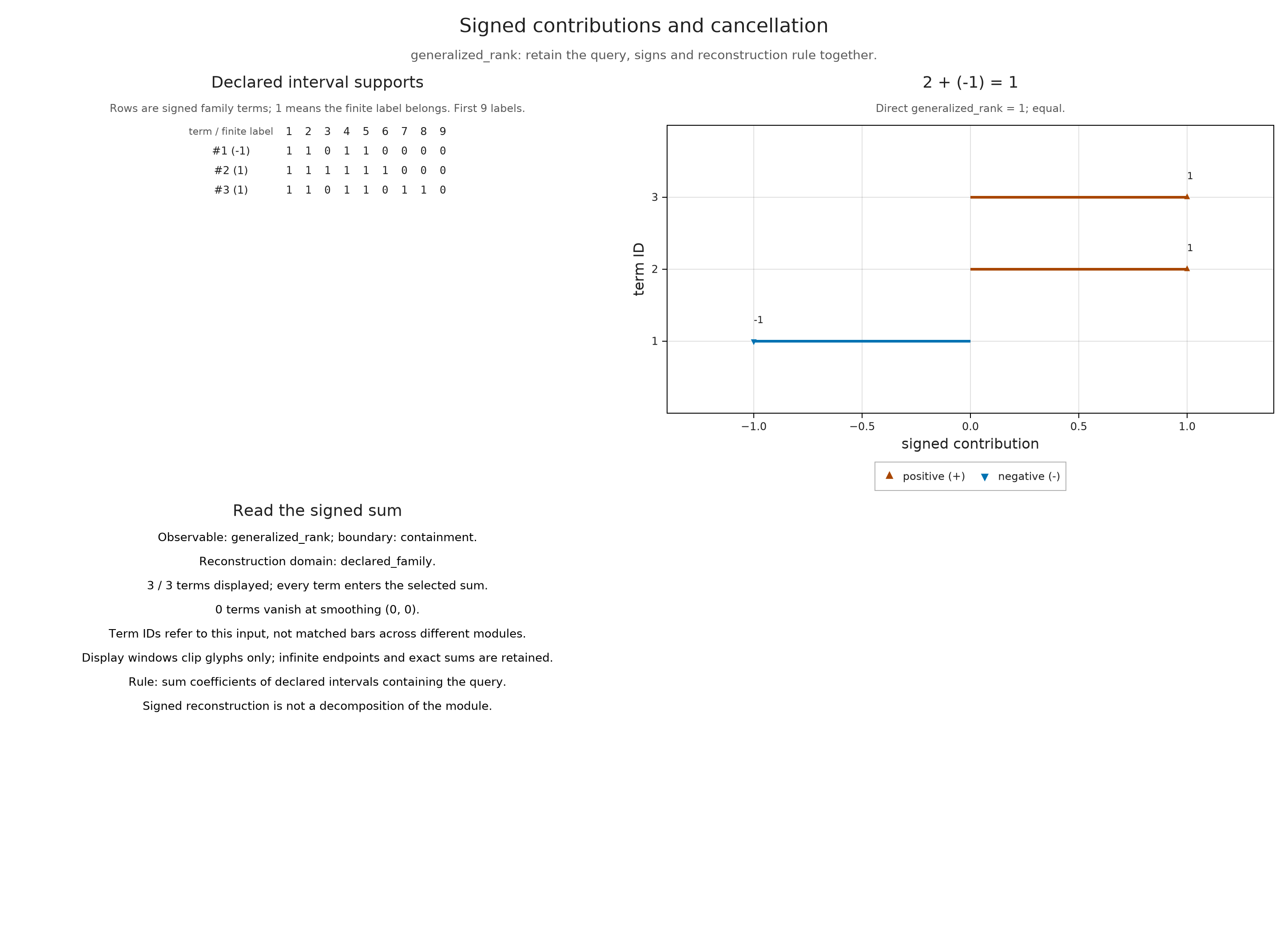
A question about a whole region can involve several branches of the order. Its generalized rank measures the image of compatible choices of vectors in their common quotient under the structure maps. The region guide develops this definition through a fork whose arrows have the same rank but different image lines.
Here we select the finite labels of the horizontal strip, the vertical strip and their overlap. Each selected region is connected by comparabilities and order convex, meaning that it contains every label between two of its labels. interval_rank_summary computes their generalized ranks and a signed reconstruction on this declared family. The table shows which labels belong to each region. Although the arithmetic resembles our rectangle calculation, this table answers only the declared region queries.
overlap = [1,2,4,5]
horizontal = [1,2,3,4,5,6]
vertical = [1,2,4,5,7,8]
family_summary = interval_rank_summary(encoding; family=[overlap,horizontal,vertical])
visualize(family_summary; query=(vertices=overlap,),
    direct=vertices -> generalized_rank(encoding; vertices))
Try moving the Hilbert query to (2,5). The correction point is no longer below the query, so only the birth term contributes and the dimension is one. For the pair query from (0,0) to (5,5), the rank is zero because the target space is zero. These checks help keep the observable in view: a signed term corrects a specified sum; it is not a submodule with a negative dimension.
What a slice window can establish
A slice follows the line $q(t)=a+td$, with basepoint $a$ and a nonzero direction $d$ whose coordinates are nonnegative. The interval endpoints are values of $t$. Rescaling $d$ changes those numbers even when the geometric line stays the same. A finite viewing window creates a second choice: do we compute only the restriction inside it, or compute the whole line and display a small part?
For this distinction, use two closed square summands, supported on $[0,2]^2$ and $[1,3]^2$. Their diagonal intervals are $[0,2]$ and $[1,3]$, with both endpoints included. Unlike our half-open grid example, a class in the first square is still present at $t=2$. The box presentation below represents the entire plane, including the zero spaces outside the squares, so it supports a query on the whole line.
box_options = A.EncodingOptions(; backend=:pl_backend,
    poset_kind=:signature, field=TamerOp.CoreModules.QQField())
closed_squares = encode([A.BoxUpset([0,0]), A.BoxUpset([1,1])],
    [A.BoxDownset([2,2]), A.BoxDownset([3,3])],
    Rational{BigInt}[1 0; 0 1], box_options)
whole_line = inspection_session(closed_squares;
    box=([3//2,3//2], [7//4,7//4]),
    slice=(basepoint=(0,0), direction=(1,1)), slice_scope=:global)
visualize(A.inspection_snapshot(whole_line))
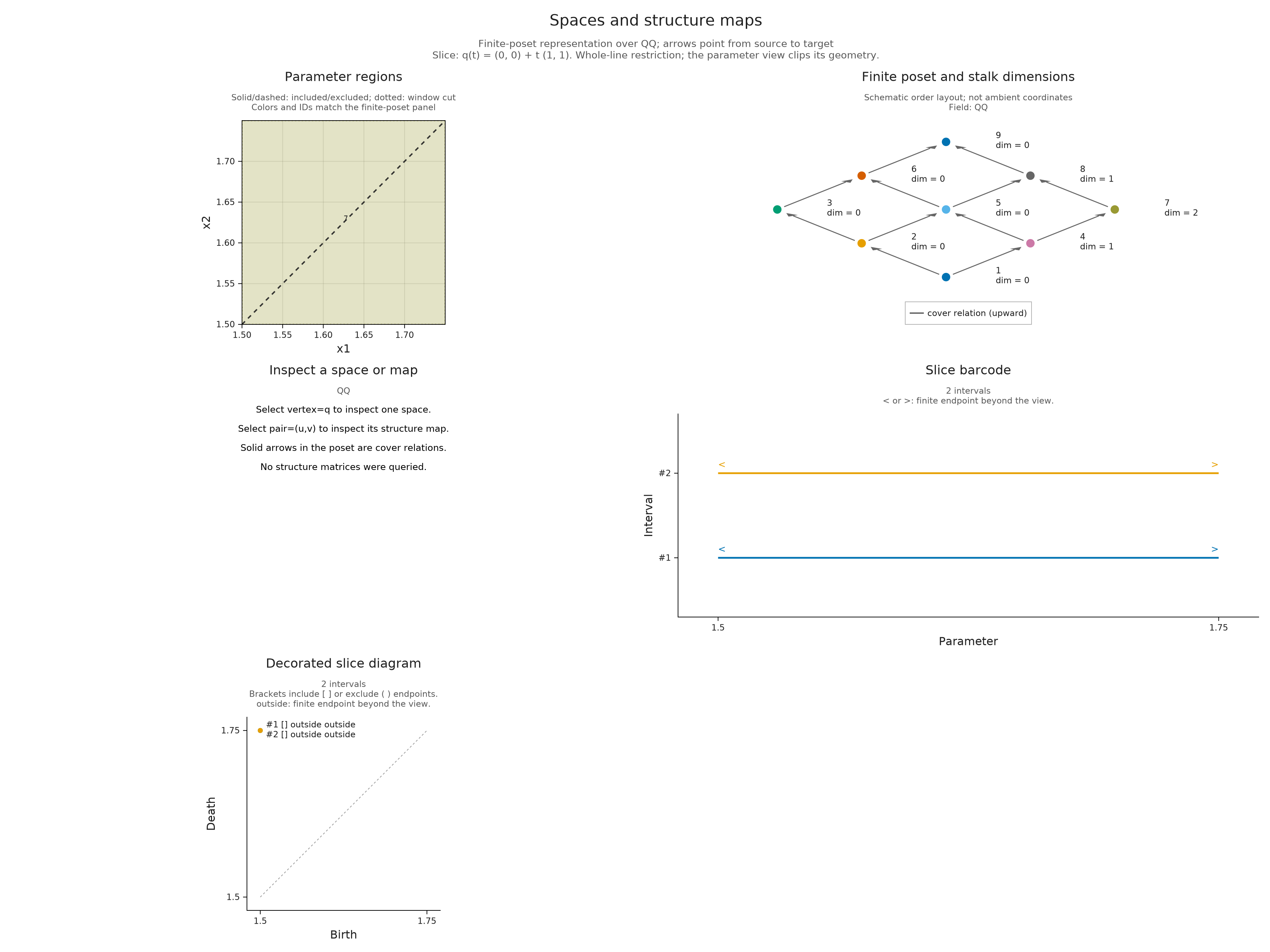
The global query knows the two different intervals even though the parameter picture shows only the part between $t=3/2$ and $t=7/4$. Change the computation to slice_scope=:window, its default, and both intervals restrict to $[3/2,7/4]$. They now form one group of multiplicity two. A question mark marks each end as censored: this restricted calculation has reached its boundary without establishing the ambient endpoint.
A.select_inspection!(whole_line; slice_scope=:window)
visualize(A.inspection_snapshot(whole_line))
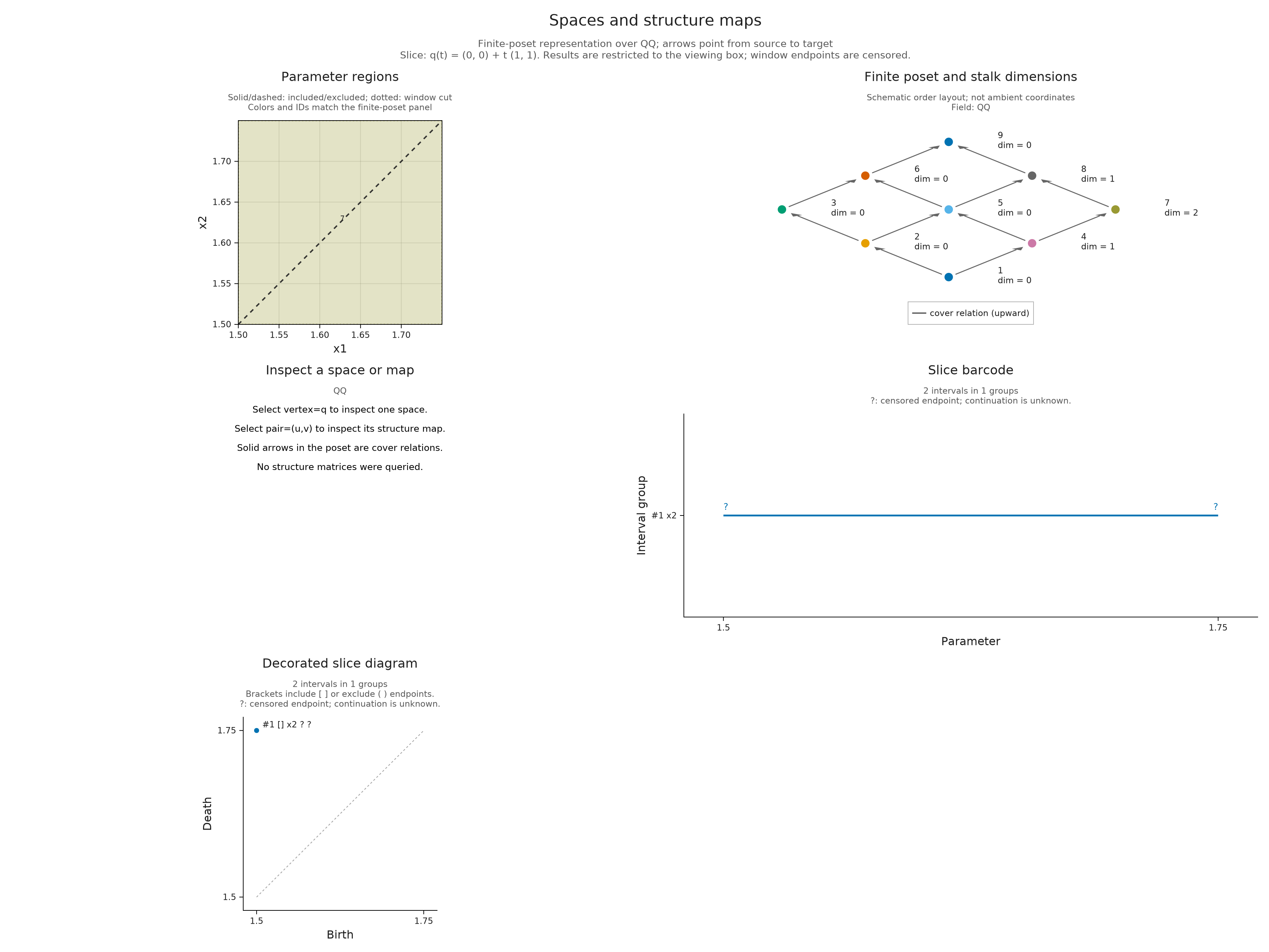
The endpoint marks distinguish the available information:
| Mark | Meaning |
|---|---|
| Filled or hollow endpoint | A finite endpoint that is included or excluded, respectively |
Continuation arrow or outside label | A known finite endpoint beyond the drawing window |
? | A boundary of the restricted computation; the ambient endpoint is unknown |
Labelled Inf or -Inf | A certified infinite endpoint |
A class present for all sufficiently large parameters can have interval $[1,\infty)$; one present on the whole line has $(-\infty,\infty)$. Infinite endpoints are never included. Neither case means merely that a finite endpoint is outside the picture. A singleton interval, present at only one parameter, is retained too: the line with basepoint (0,2) and direction (1,1) touches the two closed squares at their corners and gives $[0,0]$ and $[1,1]$.
The global calculation visits every classifier change along the line, including boundary points and the open intervals between changes. It requires all these portions of the line to be represented. A grid with unrepresented points below its first thresholds cannot be used for that request: the slice inspector does not silently add zero spaces there. Use a fully represented window for such a grid. This differs from the explicitly chosen zero extension used by the signed summaries above.
The coefficient field comes from the encoding; RealField retains its numerical rank policy. Reversed grid axes are excluded. General polyhedral classifiers require rational line and window coordinates, and reject irrational algebraic inputs. Box classifiers and supported integer extensions can describe a whole line when every required portion is represented. slice_limit, whose default is 512, bounds the number of change points and intervening open intervals before the rank calculations begin. A smaller drawing window does not reduce the work of a global query.
Translate the line through the squares
Choose one of the three parallel lines in the prepared comparison. Each uses $q(t)=(t,t+h)$, with $h=0,1,2$, so the horizontal coordinate is always the same parameter $t$. Moving the line upward shortens its intersection with each closed square. At $h=1$ the intervals are $[0,1]$ and $[1,2]$; at $h=2$ only the corner intersections remain, giving $[0,0]$ and $[1,1]$. These singleton intervals record the included corners rather than an empty intersection.
The parameter drawing uses the same window in all three views. The calculation covers the whole line, so the displayed endpoints are the actual endpoints of these square restrictions. Switch between the lines and follow each intersection into its barcode.
Explore the three parallel slices
Inspect repeated intervals
When intervals have already been computed, their inspection need not repeat persistence. This barcode has two copies of $[0,2)$, one essential interval $[1,\infty)$, and a finite interval $[8,9)$ outside the chosen display window. The two identical copies form one group with multiplicity two; the offscreen interval remains available for exact selection.
bars = Dict((0,2) => 2, (1,Inf) => 1, (8,9) => 1)
interval_session = inspection_session(bars; window=(-1,4))
visualize(A.inspection_snapshot(interval_session))
![The barcode shows two copies of [0,2) and the essential interval [1,Inf) within the display window. The separate interval [8,9) lies outside the picture and remains in the retained result.](slices_diagrams_files/slices_diagrams_27_0.png)
Moving a slice
Optional: moving a slice
With WGLMakie loaded and Julia running, use the same square encoding to open a movable line:
using WGLMakie
slices = inspection_session(closed_squares; box=([-1,-1],[4,4]),
    slice=(basepoint=(0,0), direction=(1,1)))
visualize(slices; backend=:wglmakie)
A.select_inspection!(slices;
    slice=(basepoint=(0,1), direction=(1,1)))
The translated line gives $[0,1]$ and $[1,2]$. The first square handle translates the line and the second changes its direction; the angle and offset sliders provide keyboard control. Horizontal and vertical directions are allowed. Read the displayed equation when comparing endpoints, because moving a handle can change the origin or scale of $t$ as well as the line. Text fields accept exact fractions. Sliders use decimal approximations, and releasing a handle rounds its coordinates to ten decimal places.
Turn off Continuous slice updates to choose a slider position before computing, or enter exact coordinates and press Apply slice. While a request is pending, the message distinguishes the requested line from the result still visible. The Slice scope selector switches between the window and global queries described above; press Apply slice to commit it.
Click an interval or diagram point to highlight its group in both charts and its segment in the parameter plane. Intervals with the same endpoints and inclusion flags share a group and multiplicity; repeated clicks on coincident points cycle through distinct groups. The Selected interval group selector reaches retained groups outside the drawing budget or window. Changing the line or scope clears the interval selection because a group on one slice does not identify a class on another. The independent stalk or map selection remains.
Previously queried lines can be reused from a bounded cache, while a new line may require materializing a lazy module and computing ranks. Selection among the current intervals reuses their result. Once finished, A.close_inspection!(slices) releases the live session; its final snapshot remains available.
Interval members and sharing
Optional: interval members and sharing
Render interval_session with WGLMakie to inspect its groups interactively:
visualize(interval_session; backend=:wglmakie)
A.select_inspection!(interval_session; interval=1)
A.inspection_summary(interval_session)
The same workflow accepts ordinary diagrams, raw interval vectors or dictionaries, packed barcodes, and selected results from a slice family. Supply index when a family has several barcodes and dim when choosing the homological degree of an ordinary diagram. Superlevel intervals continue toward smaller parameter values, with essential intervals ending at -Inf.
An ordinary diagram computed with representatives=true can distinguish original members of a repeated interval by their retained cycles. Choose Original member number before requesting Show retained representative, or pass member=j, representative=true when selecting the interval. Changing the group or member clears that request unless it is supplied again. Endpoint data alone cannot recover a cycle; the source cell guide explains retention, coefficients and fillings, including repeated periodic classes. Such representatives depend on choices in the reduction and need not be canonical or geometrically shortest.
For signed terms, the corresponding live view starts with inspection_session(rank_measure; query=(p=(0,0), q=(2,2)), direct=direct_rank). Changing a term reuses the answer; changing the query or smoothing asks for a fresh direct comparison. Invalid edits keep the previous snapshot. In a static export, max_terms limits drawn terms while reconstruction still sums every retained coefficient.
save_visual("signed-rank.svg", signed_view; backend=:cairomakie) saves the prepared signed answer. A live session can be saved through A.inspection_snapshot(session), which retains the selected picture and readout without callbacks. To compare two barcodes and see which pairs determine their distance, continue with the matching witness recipe. The visualization reference gives the exact signed-view contracts.
Prepare the slice comparisons
Optional: Prepare the slice comparisons
The following cell computes the three lines used above and checks their intervals against the square intersections. Each named view keeps its parameter picture, finite order, barcode and diagram together. visual_panel selects these drawings from the snapshot; the general inspector readout is unnecessary for this comparison. Saving the collection prepares the same choices for a browser.
prepared_slices = inspection_session(closed_squares; box=([-1,-1], [4,4]),
    slice=(basepoint=(0,0), direction=(1,1)), slice_scope=:global)
slice_views = Pair{Symbol,Any}[]
for offset in 0:2
    A.select_inspection!(prepared_slices;
        slice=(basepoint=(0,offset), direction=(1,1)))
    snapshot = A.inspection_snapshot(prepared_slices)
    intervals = snapshot.metadata.slice_result.intervals
    @assert Set((r.birth, r.death, r.left_closed, r.right_closed, r.multiplicity)
        for r in intervals) == Set(((0, 2-offset, true, true, 1),
                                   (1, 3-offset, true, true, 1)))
    @assert all(r -> r.singleton == (offset == 2), intervals)
    picture = TamerOp.compose_visuals((
        parameters=TamerOp.visual_panel(snapshot; panel=:region_labels),
        order=TamerOp.visual_panel(snapshot; panel=2),
        barcode=TamerOp.visual_panel(snapshot; panel=:slice_barcode,
            limits=(x=(-1,4), y=(0,3))),
        diagram=TamerOp.visual_panel(snapshot; panel=:slice_diagram,
            limits=(x=(-1,4), y=(-1,4))));
        columns=2, title="q(t) = (t, t + $offset)",
        subtitle="Rational square modules; whole line restriction; closed endpoints")
    push!(slice_views, Symbol("Offset h = $offset") => picture)
end
mkpath(joinpath("tamerop_outputs", "slices"))
TamerOp.save_visual_session(joinpath("tamerop_outputs", "slices", "parallel_lines.html"),
    (; slice_views...); title="Translate a line through two closed squares",
    caption="Choose h in q(t) = (t, t + h). The squares are [0,2]² and [1,3]² over the rational field. Each query covers the whole line; filled endpoints include the corners. The parameter and barcode windows stay fixed.", size=(1200,1000))
A.close_inspection!(prepared_slices);
A.close_inspection!(whole_line)
A.close_inspection!(interval_session);