Exact rhomboid multicover construction
Take two sites at $(0,0)$ and $(2,0)$ and grow closed balls around them. At radius one, a location first belongs to both balls, and their union becomes connected. The same event is seen at two coverage depths. A finite model of multicover must describe these spaces together with the maps obtained by increasing radius or decreasing the required depth.
TamerOp builds a graded cellular complex: cells with boundary maps and grades specifying when they appear. It can then encode the homology over a finite parameter poset. The geometric inspector retains this same complex before encoding, so it can relate a selected cell to the source sites and its birth. We will follow the construction from site labels through exact radii to signed boundaries. The multicover guide computes the two-site example and a square whose loop eventually fills.
From spheres to cells
A separating sphere partitions the indexed sites into an inside set $I$, an on-sphere set $O$ and the remaining outside sites. The native rhomboid has label $(I,O)$ and dimension $|O|$. The general position hypothesis excludes extra cospherical sites in the relevant geometry, so the on-sphere directions give it the face structure of a cube. Moving one site from $O$ into $I$, or from $O$ to the outside, chooses one of the two opposite faces in that direction. Shared faces are identified by these labels.
This is the rhomboid model of Corbet, Kerber, Lesnick and Osang, Section 4. Its vertices correspond to subsets $S$ with $I\subseteq S\subseteq I\cup O$. For sites $a_i$, the inspector places them at
\[v_S=\left(\sum_{i\in S}a_i,\ |S|\right).\]
The last coordinate counts sites and gives positive depth; reflecting it recovers the usual negative depth convention. Thus planar input has a cell model in three dimensions. The spatial coordinate is a sum, so dividing it by depth to obtain a mean would change this geometry. Projecting away depth changes the drawing, whereas selecting a depth section changes the complex.
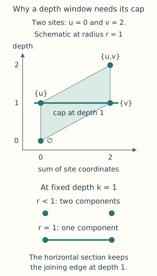
In this schematic the sites lie on a line, so the lifted cell has two coordinates. The full rhomboid has the four subset vertices shown. Cutting at depth one gives a joining edge that is absent before its birth radius; it is a new face of the sliced model.
Exhaustive discovery enumerates affinely independent supports containing one more site than the affine dimension. It solves for circumspheres and classifies the sites with rational arithmetic in the original Euclidean metric, even when the cloud lies in an affine subspace of smaller dimension. Faces are inserted recursively and shared through their labels. Extra cospherical sites in relevant geometry violate the native contract and cause an error, rather than an arbitrary choice of diagonal or a perturbation of the sites.
An alternative route discovers the labels across successive depth levels. Both routes feed the same radius and boundary construction; we return to that discovery algorithm below after explaining what its cells must retain.
A birth radius is a constrained minimum
Fix a label $(I,O)$. A realizing sphere must touch the sites of $O$, enclose those of $I$ and leave the outside sites outside. The smallest sphere through $O$ alone may violate one of the other conditions. If so, a minimum subject to all the conditions can occur where another site becomes tight, placing it on the sphere of a coface, a larger cell containing the original one.
The implementation therefore works from higher dimensions downward. It accepts an unconstrained circumradius when its exact site classification is feasible, then passes each coface's minimum to its faces and keeps the least feasible squared radius. The empty anchor vertex has radius zero. If a required realizing coface is missing, the constructor reports an error.
These squared radii are rational. The constructor takes an exact algebraic square root when emitting grades, so $r^2=2$ becomes $r=\sqrt2$ with equality preserved at the birth event. Finite floating inputs are interpreted as their exact binary rational values. A radius cutoff is converted exactly before squaring; multiplying it in floating arithmetic first could change the boundary being requested. The inspector reports both radius and squared birth radius while selecting cells with the physical radius parameter.
Incidence, windows and finite encodings
Ordering the sites of $O$ orients each cube. Removing a direction gives two facets with opposite boundary coefficients, and the sign alternates across directions. A shared face has one identity in the boundary matrix. These integer coefficients can be used over any admitted coefficient field without reconstructing an orientation from a polygon drawn on screen.
A cell in the unsliced model has grade $(\rho(I,O),|I|)$, where $\rho$ is its constrained birth radius. For a bounded depth window, the constructor takes horizontal sections at integer depths and closed slabs between them. It does this before imposing max_dim, since a higher dimensional cell can contribute a cap of one lower dimension. The two-site window (1,1) consists of the horizontal section in the figure: its joining edge survives although no slab of positive width does. The depth guide gives the radius pruning argument, cap comparison and signed boundary formulas.
A request for stage=:simplex_tree additionally subdivides the cells. For unsliced cubes, a Freudenthal triangulation takes each ordering of the cube directions and follows the chain of subset vertices obtained by adding them in that order. Shared faces use the same global vertex labels and agree on their subdivision. Bounded depth cells instead use flags in their actual face poset: a strict chain of faces gives a simplex with its largest face's grade. These subdivisions can be much larger. Graded complex, encoding and geometric inspection requests keep the cellular representation.
With grades and boundaries fixed, increasing radius or decreasing depth includes one subcomplex in another. Homology of these inclusions supplies the module's structure maps. Encoding organizes the spaces and maps on a finite grid; geometric inspection itself does not materialize that encoding. Custom axes can move births to earlier grid samples by floor placement. The inspector uses the original cell grades, so a comparison with such an encoding must account for the changed filtration.
Discover cells across depth levels
backend=:incremental starts with singleton labels at depth one and obtains labels needed at later depths from the cells it has already found. For a subset $Q$ of $k$ sites, form the lifted point
\[\left(\frac1k\sum_{a\in Q}a,\ \frac1k\sum_{a\in Q}\lVert a\rVert^2\right).\]
The convex hull is the smallest convex set containing these lifted points. Its lower faces, viewed in the spatial coordinates, give the cells of a weighted Delaunay mosaic. Each vertex keeps its subset label. For a cell at depth $k$, intersect its labels to obtain $I$ and subtract $I$ from their union to obtain $O$. Its generation is $k-|I|$; cells of generation one are the sections one level above the anchor of a newly discovered rhomboid. That rhomboid supplies subset vertices at later depths. The discovery theorem ensures that those earlier cells provide all the vertices needed for the next level, so the algorithm need not enumerate every subset of the input. This is the construction of Edelsbrunner and Osang, Theorem 5, Lemma 2 and Algorithm 1.
TamerOp uses CDD's exact rational conversion between convex hull vertices and defining inequalities, adding an upward vertical ray to the lifted hull and selecting facets with negative final normal coefficient. This includes the case where the lifted vertices of a simplex lie in one affine plane. CDD returns whole facets, so higher generation cells that are not simplices require no arbitrary triangulation. Recovered top rhomboids are checked against exact sphere classifications.
For a cloud in a proper affine subspace, an injective coordinate projection reduces the horizontal coordinates of the lifted hull. The final coordinate still uses the original full squared norm, preserving the input's Euclidean metric. Means, facet incidence and sphere classification all remain exact.
The algorithm stops at the requested upper depth, or sooner if no new top rhomboids are possible. It must still process prerequisite levels below lo. Here incremental refers to discovery across depths. CDD recomputes a weighted hull at each level, so the cost includes this geometry work as well as producing the output cells. This use of a convex hull is among the weighted Delaunay methods allowed in Corbet and collaborators, Section 4.5. The guide states the supported dimensions, general position requirements and automatic selection rule beside the user's backend choice.
Retaining geometry without changing the model
filtered_complex requests geometry from the same constructor that emits the graded complex. Native cells retain $(I,O)$, squared radius and any section or slab identity. Section vertices are lifted subset vertices at the retained integer levels. The boundary order of a two dimensional face is found by walking its actual edges with exact vertex equality. It is therefore already known before any drawing is made.
For degenerate input, :subdivision_cech instead emits simplices whose vertices are labelled subsets and whose simplices are strict inclusion flags. Their subset means and cardinalities give a schematic layout for inspection. Two diagonals of a square share a mean; repeated labelled sites can coincide too. The layout can therefore overlap while the cell identities and boundaries remain distinct. This is a different model from a native rhomboid tiling. Its relation to multicover comes from the diagrammatic subdivision–Čech argument of Blumberg and Lesnick, Theorem 4.13 and Remark 4.14.
For the closed Euclidean balls used here, the closed-cover hypotheses continue to hold at exact births, including singleton intersections. Nested closed convex sets have the homotopy extension property: a homotopy on the smaller set, compatible with an initial map on the larger one, extends to the larger set. This supplies the extension condition needed for the comparison; see Bauer, Kerber, Roll and Rolle, Theorem 5.9(1b), Corollary 5.16 and Proposition 5.19. Repeated sites remain indexed by label subsets even when the geometric sets coincide, allowing the same comparison by unions of labels. Deduplicating those indices would change coverage. At depth zero, the empty subset supplies the cone and the comparison with ambient space. The equivalence respects maps in both parameters. For native rhomboids, the corresponding comparison and its bounded terminal attachment are explained in the depth guide.
The source panel counts indexed balls through exact squared-distance tests at its display sample points. A thin or singleton intersection can fall between those samples, so the raster is never used to compute homology. For source data in more than two dimensions, the panel evaluates a declared spatial section: circle outlines are sections of spheres, while site markers are projected.
At a selected parameter, homology uses the active submatrices of the retained boundary maps. Over the chosen field,
\[\beta_d=\dim C_d-\operatorname{rank}\partial_d- \operatorname{rank}\partial_{d+1},\]
where $C_d$ is the vector space generated by active cells of dimension $d$, and $\partial_d$ is its boundary map. Display budgets omit drawn cells but leave this complex unchanged; separate algebra budgets can reject oversized rank or reduction requests. At fixed depth, a barcode uses each retained cell's earliest allowed radius and its existing boundary column, with a prime coefficient field. A finite radius cap censors intervals that still survive there, giving no conclusion about their eventual death in the uncapped model.
Reuse and where the work grows
An explicit SessionCache can keep exact geometry between requests. Its retained original cells are the carriers from which later outputs are built. Native entries depend on coordinate contents and shape, requested backend and depth window. Radius cutoffs, output skeletons, fields, degrees, axes and output stages can reuse compatible carriers. Subdivision–Čech entries retain exact subset minimum-ball radii for the coordinates and lower depth bound; changing the upper bound changes the emitted grades. The constructions have separate entries. Returned geometry and complexes own their mutable arrays, so editing a result leaves the retained geometry unchanged.
Concurrent first requests publish one complete result under the session's encoding cache lock, which also protects clearing. CDD execution has a separate boundary shared with piecewise linear geometry; the concurrency contract explains its external-call and configuration limits. The first lock governs sharing in the session; the second governs execution in CDD. Input clouds must not be modified while another task is reading them.
cache=:auto supplies a cache for one call, and cache=nothing disables geometry reuse. Reuse across calls needs an explicit session. Distinct coordinate, window and backend entries remain until the session is cleared or discarded, so repeated edits in a long session can accumulate storage. Budget checks apply again on a cache hit, including recorded workspace peaks and the requested slicing or subdivision, but do not bound aggregate session memory. The notebook shows two requests sharing one session.
Exhaustive discovery spends work enumerating sphere supports and their faces; incremental discovery spends it on exact weighted hulls. Both also pay for rational geometric decisions and constrained radius propagation. Flag subdivision can grow exponentially even for a small cloud, which makes its explicit cell budget consequential. Inspection adds stored vertices, scans for active cells and membership queries at drawing samples. Boundary ranks and barcode reduction can take more work than those display operations.
These costs concern different parts of the same construction. Comparing enumeration methods requires identical data and depth windows; comparing full and capped models additionally changes the emitted cell structure. Exact integer sizes and CDD's native memory matter alongside Julia's allocations. Versioned benchmark reports supply measured comparisons under their stated conditions.
See the implementation bibliography for the mathematical and algorithmic sources.