Computing Ext, Tor and their products
Download the executed notebook · Build and environment record
A finite module retains linear maps between its spaces, which lets us ask how it relates to other modules. Hom describes compatible maps. Ext extends that question: in degree 1 it describes short exact sequences with the two modules at their ends, and higher degrees allow longer extensions. By computing representatives of these classes, we can follow what happens when extensions compose.
We begin with the four simple modules on a diamond, count their Ext classes and examine two products in the same target group. Later, Tor will give a reason to pay attention to which way the module maps run and to the additional data needed for multiplication. You should be comfortable with vector spaces, linear maps and quotients by subspaces. The resolution guide develops the projective resolution behind our first calculation.
All computations use rational coefficients and belong to the category of modules on the supplied finite poset. OP.ext accepts an EncodingResult by using its finite module and base, but recovery of an ambient persistence module does not identify its ambient Ext with these groups. The category discussion explains that comparison, and the reference gives the precise calling conventions.
import TamerOp as OP
import CairoMakie
using SparseArrays: sparse

field = OP.CoreModules.QQField()
P = OP.Advanced.FinitePoset(Bool[1 1 1 1; 0 1 0 1; 0 0 1 1; 0 0 0 1])
OP.visualize(P)
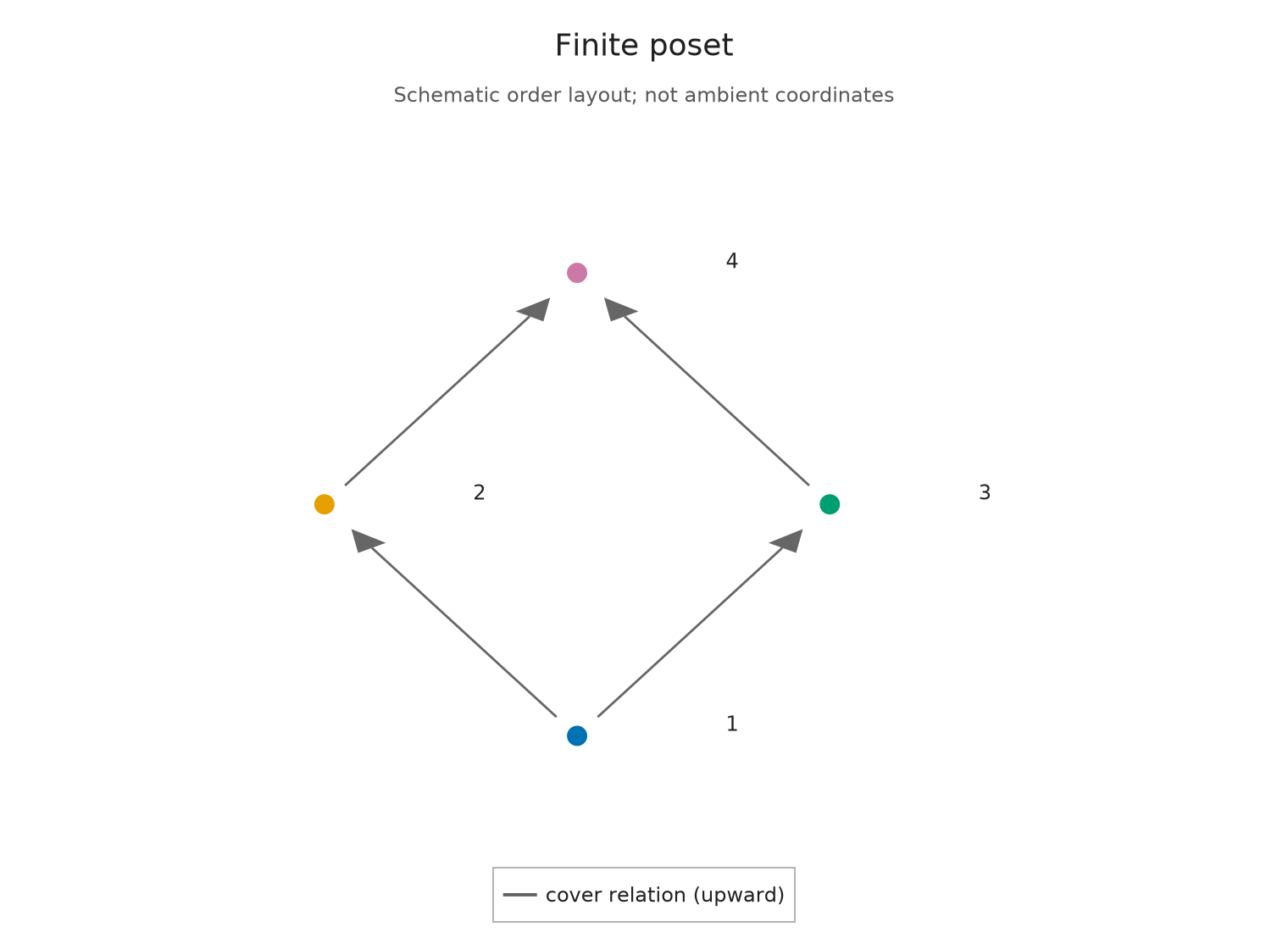
A small category with two routes
Let $S_i$ have the field $K=\mathbb Q$ at vertex $i$ and zero at the other vertices. All cover maps are zero. These are the four simple modules, meaning their only submodules are zero and themselves. The shape of each zero matrix still matters: a map from a line to zero has zero rows and one column.
We can predict $\operatorname{Ext}^*(S_1,S_4)$ from the resolution
\[0\longrightarrow P_4\longrightarrow P_2\oplus P_3 \longrightarrow P_1\longrightarrow S_1\longrightarrow0,\]
where $P_i$ is the principal projective at vertex $i$. A map from $P_i$ to $S_4$ is determined by a vector in the stalk of $S_4$ at $i$, so only $\operatorname{Hom}(P_4,S_4)$ is nonzero. Applying Hom therefore gives a complex with one copy of $K$ in degree 2 and zero elsewhere. Its cohomology, and hence Ext, has dimensions 0, 0 and 1 in degrees 0, 1 and 2.
There are degree 1 classes from $S_1$ to $S_2$ and from $S_2$ to $S_4$, as well as analogous classes through $S_3$. We will compare the products along these two routes.
stalks = [[Int(v == i) for v in 1:4] for i in 1:4]
simples = [OP.Advanced.PModule{OP.QQ}(P, dims,
    Dict((u,v) => zeros(OP.QQ, dims[v], dims[u]) for (u,v) in OP.Advanced.cover_edges(P)); field)
    for dims in stalks]
S1, S2, S3, S4 = simples
E14 = OP.ext(S1, S4; maxdeg=2)
OP.visualize(E14)
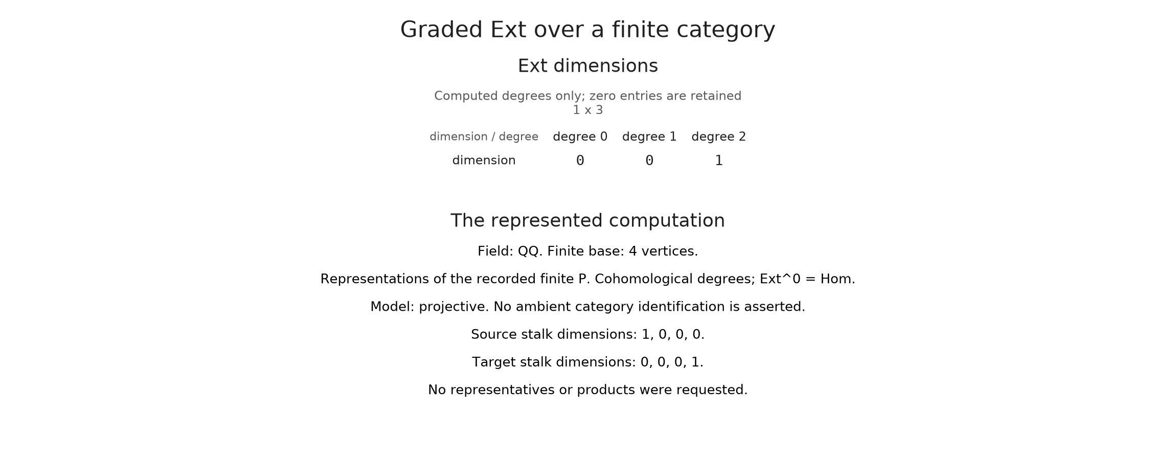
The result agrees with that calculation. Degree 0 is ordinary Hom, while degree 2 contains one independent extension class. A displayed zero means the group was computed and found to vanish; degrees outside the requested range are still uncomputed.
At this point we have asked for dimensions. If later calls should reuse compatible resolutions, create sc = OP.SessionCache() and pass cache=sc. Reuse concerns the stored calculation; the finite category and the meaning of a quotient coordinate still have to agree.
OP.describe(E14)
(kind = :ext_space, model = :projective, provenance = (category = :finite_poset_representations, base_poset = FinitePoset(nvertices=4), field = TamerOp.CoreModules.CoeffFields.QQField(), degree = 0:2, degree_convention = :cohomological, model = :projective, orientation = :forward, argument_variance = (:contravariant, :covariant), ambient_identification = :not_asserted), field = TamerOp.CoreModules.CoeffFields.QQField(), nvertices = 4, degree_range = 0:2, nonzero_degrees = (2,), degree_dimensions = Dict(2 => 1), total_dimension = 1)From a class to a representative
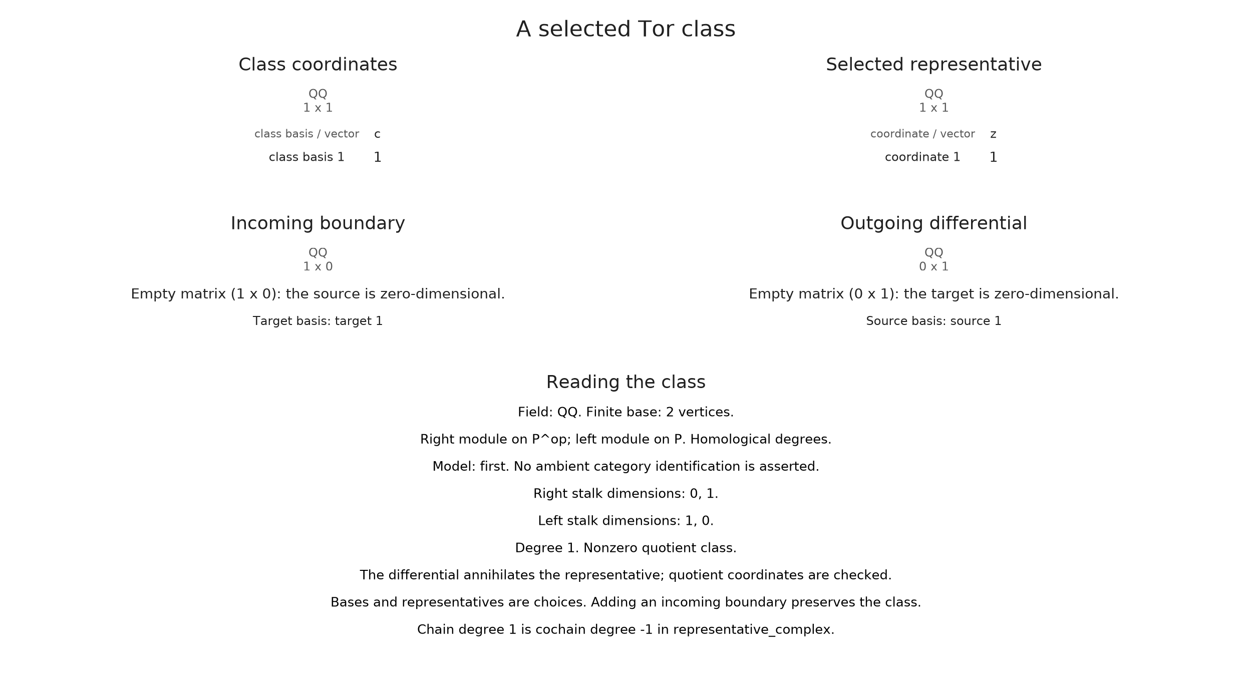
An Ext class is a cocycle modulo coboundaries in a Hom complex. A cocycle is killed by the next differential, and a coboundary is in the image of the previous one. Their quotient identifies different cocycles representing the same extension class.
In this one-dimensional Ext group, vector=[1] selects the first quotient basis vector. These are coordinates of a class, rather than coordinates in a stalk of $S_1$ or $S_4$. The figure places a representative beside the adjacent differentials so we can inspect both the cycle equation and the quotient calculation.
OP.visualize(E14; kind=:derived_class, degree=2, vector=[1])
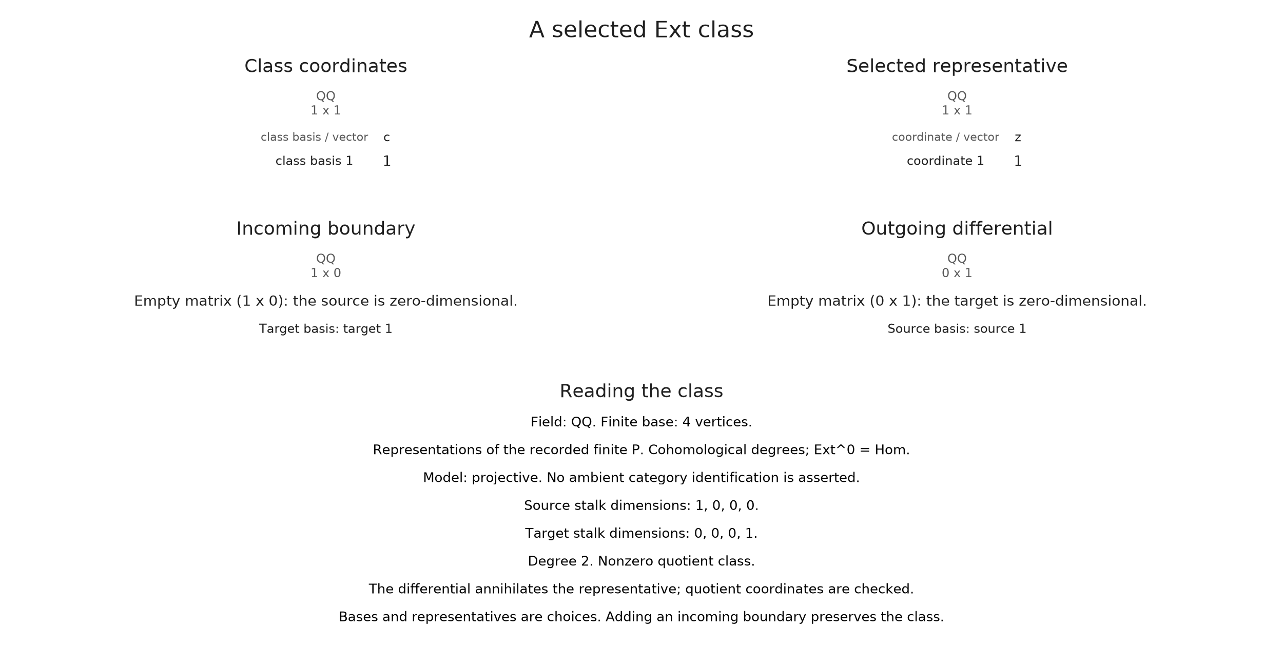
The specification retains the representative and checks that its differential vanishes and its quotient coordinates agree with the selection. The following inspection reads those checks together with the exact coordinates. On a larger example, the chosen representative could differ from another cocycle by an incoming boundary; the complex guide follows that difference explicitly.
class_view = OP.Advanced.visual_spec(E14; kind=:derived_class, degree=2, vector=[1])
selection = class_view.metadata.selection
@assert selection.cycle_equation.valid
@assert selection.coordinate_equation.valid
selection.coordinates
1-element Vector{Rational{BigInt}}:
 1
Compose along the two routes
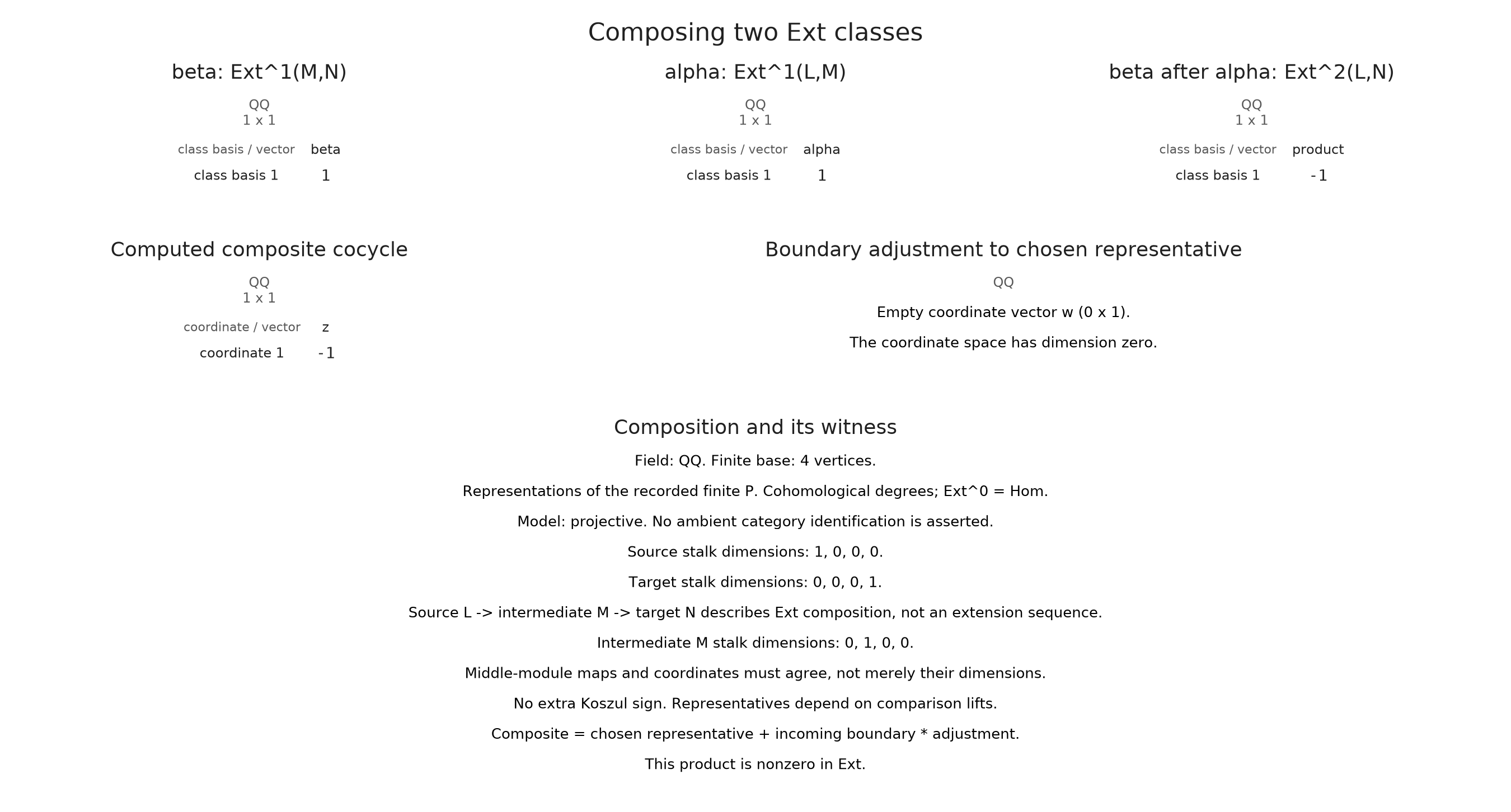
Choose $\alpha\in\operatorname{Ext}^1(S_1,S_2)$ and $\beta\in\operatorname{Ext}^1(S_2,S_4)$. Their Yoneda product $\beta\alpha$ lies in $\operatorname{Ext}^2(S_1,S_4)$. The left factor acts after the right factor, as in matrix composition. In terms of extensions, this joins two short exact sequences; the computation represents the resulting class using a lift between projective resolutions.
That lift reaches degree 2 in the resolution used by the right factor, even though the right class itself has degree 1. We therefore compute E12 through degree 2. Supplying target=E14 expresses the product in the target basis already chosen above. The figure displays the computed cocycle and its class, without constructing a sequence of extension modules.
E24 = OP.ext(S2, S4; maxdeg=1)
E12 = OP.ext(S1, S2; maxdeg=2)
via2 = OP.Advanced.visual_spec(E24; kind=:yoneda_product,
    right=E12, p=1, q=1, left_vector=[1], right_vector=[1], target=E14)
OP.visualize(via2)
E34 = OP.ext(S3, S4; maxdeg=1)
E13 = OP.ext(S1, S3; maxdeg=2)
via3 = OP.Advanced.visual_spec(E34; kind=:yoneda_product,
    right=E13, p=1, q=1, left_vector=[1], right_vector=[1], target=E14)
c2 = via2.metadata.selection.coordinates
c3 = via3.metadata.selection.coordinates
@assert c2 != [0]
@assert c2 == -c3
(c2, c3)
(Rational{BigInt}[-1], Rational{BigInt}[1])Both products are nonzero, and their coordinates have opposite signs in the same target basis. This is the signed relation coming from the diamond's commutative square: in the resolution of $S_1$, the two degree 1 generators meet at vertex 4 with a relation having opposite coefficients. The multiplication call uses the signs in those differentials without inserting an extra sign afterward.
The coefficient of an individual product depends on our chosen basis classes. Comparing both products in E14 makes the displayed relation meaningful. Over a field of characteristic 2, opposite coefficients coincide, so the same relation is written with equal coefficients.
Bilinearity gives another prediction we can check without finding new lifts by hand: replacing the left class by zero makes its product zero.
zero_product = OP.Advanced.visual_spec(E24; kind=:yoneda_product,
    right=E12, p=1, q=1, left_vector=[0], right_vector=[1], target=E14)
@assert zero_product.metadata.selection.zero_class
zero_product.metadata.selection.coordinates
1-element Vector{Rational{BigInt}}:
 0
Compare the products in one target basis
Choose the route through vertex 2, the route through vertex 3, or the zero left factor. The two nonzero products have opposite coordinates in E14; the zero factor gives zero. Keeping that target basis fixed lets us read the sign relation directly, while the preceding representative calculation explains where it comes from.
Compare the two routes and the zero product
Asking for several extension products together
When several selected combinations are needed, place their coordinate vectors in matrix columns. We can keep the route through vertex 2 and choose left classes with coordinates 1, $-1$ and 0, together with right classes with coordinates 1 and 2. Bilinearity predicts the six answers from the product already computed.
The result has three indices: products[:,j,i] gives the target coordinates for left column j composed with right column i. We display its only target coordinate as a matrix, whose rows now index the chosen left classes and columns the chosen right classes.
left_columns = reshape(OP.QQ[1,-1,0], 1, 3)
right_columns = reshape(OP.QQ[1,2], 1, 2)
product_target, products = OP.Advanced.yoneda_product(
    E24, 1, left_columns, E12, 1, right_columns; ELN=E14)
@assert size(products) == (1,3,2)
@assert products[1,:,:] == c2[1] * OP.QQ[1 2; -1 -2; 0 0]
products[1,:,:]
3×2 Matrix{Rational{BigInt}}:
 -1  -2
  1   2
  0   0
Identity matrices as inputs would select every basis class. Other matrices, such as these, select only the combinations we supply. The right resolution must still reach the sum of the two degrees, and all columns use the coordinate bases of their respective Ext results. ELN=E14 fixes the target coordinates; if a supplied target uses a different projective resolution of the same modules, a comparison lift transfers the result into that model.
The computation lifts each right class once and reuses that lift with all selected left classes. Those lifts last for this call. With return_cocycle=true, a third return value contains the actual cocycles with the same two column indices; its first index instead runs over cochain coordinates in the returned target model. Over exact fields these coordinates agree exactly with separate scalar calls. Numerical fields use their declared tolerances.
Compute a whole degree pair when it is useful
For repeated multiplication in a single Ext algebra, we can retain a table of products of basis classes. Put the four simple modules together as $M=S_1\oplus S_2\oplus S_3\oplus S_4$. Its stalk is one-dimensional at each vertex, but every cover map is zero. A constant module would have identity cover maps, so it would be a different input despite having the same dimensions.
The self-Ext dimensions of $M$ are 4, 4 and 1. In degree 0 there is one identity for each simple; in degree 1 there is one class for each of the four covers; and degree 2 contains the class joining bottom to top. An ExtAlgebra keeps a projective self-Ext model and stores a multiplication table when a degree pair is requested.
The default view reads dimensions. Requesting kind=:product_table computes the selected pair. Its columns index ordered pairs of basis classes, with the right index varying fastest, and its rows give target coordinates. Here we display all sixteen columns so the two nonzero products can be compared.
M = OP.Advanced.PModule{OP.QQ}(P, ones(Int,4),
    Dict(edge => zeros(OP.QQ,1,1) for edge in OP.Advanced.cover_edges(P)); field)
finite = OP.EncodingResult(P, M, nothing)
A = OP.ext_algebra(finite; maxdeg=2)
OP.visualize(A; kind=:product_table, p=1, q=1, matrix_limit=(1,16))
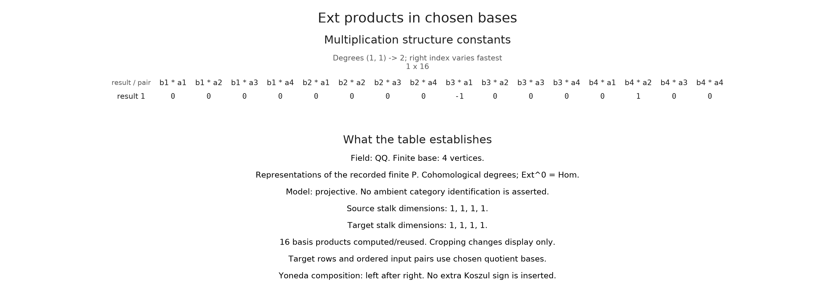
Only the two composable routes across the diamond give nonzero products among these sixteen pairs. Their coefficients cancel, as in the comparison above. A completed table can be reused by later multiplications in the same algebra.
The request limits the amount of table data it is prepared to compute: by default, max_products=4096 bounds the number of input basis pairs and max_entries=1_000_000 bounds the number of output coefficients. Those bounds are separate from matrix_limit, which controls how much of an already computed table is drawn.
constants = OP.Advanced.multiplication_matrix(A, 1, 1)
@assert size(constants) == (1,16)
@assert count(!iszero, constants) == 2
@assert sum(constants) == 0
OP.Advanced.cached_product_degrees(A)
1-element Vector{Tuple{Int64, Int64}}:
 (1, 1)
Induced maps use declared coordinates
A module map $f:M'\to M$ induces a map $\operatorname{Ext}^t(M,N)\to\operatorname{Ext}^t(M',N)$ by precomposition. This reversal is what contravariant in the first argument means. A map $g:N\to N'$ induces a map in the same direction on the second argument, which is covariance.
For an endomorphism of $S_1$ multiplying its line by 2, precomposition multiplies $\operatorname{Ext}^2(S_1,S_4)$ by 2. Since the source and target are the same module, this example keeps the direction unobtrusive while making the induced matrix easy to predict. With distinct modules, the Ext models must match the displayed variance and their coordinate choices; matching dimensions does not suffice.
twice = OP.Advanced.PMorphism(S1, S1,
    [2 * ones(OP.QQ,d,d) for d in stalks[1]])
induced = OP.Advanced.ext_map_first(E14, E14, twice; t=2)
@assert induced == reshape(OP.QQ[2],1,1)
induced
1×1 Matrix{Rational{BigInt}}:
 2
Tor pairs opposite actions
The incidence algebra of a finite poset encodes its comparable pairs and their composition. Tensoring over this algebra pairs a right module with a left module. TamerOp represents the right module as a forward diagram on $P^{\mathrm{op}}$, the same vertices with reversed order, and the left module as a diagram on $P$.
On the chain $1<2$, put the right module $R$ at vertex 2 and the left module $L$ at vertex 1. A projective resolution of $R$ on the opposite chain has the principal projective at 2 in degree 0 and the one at 1 in degree 1. Tensoring a principal right projective at $i$ with $L$ gives $L_i$, so the tensor complex is $K\to0$ in degrees 1 and 0. Its homology is therefore one-dimensional in degree 1 and zero in degree 0.
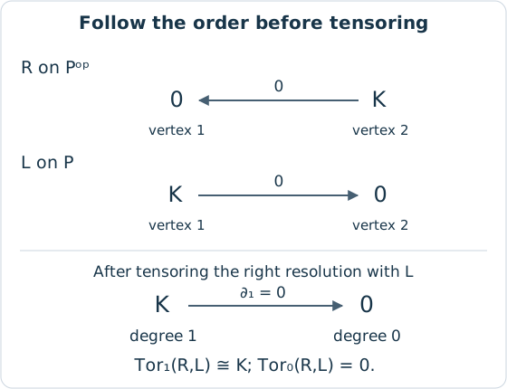
This calculation uses the tensor product over the incidence algebra. The pointwise tensor of two forward modules is a different operation. Tor uses homological degrees, with boundaries lowering degree; its representative view keeps those labels even though the shared complex inspector uses the equivalent indexing $C^{-s}=C_s$.
Q = OP.Advanced.FinitePoset(Bool[1 1;0 1])
Qop = OP.Advanced.FinitePoset(Bool[1 0;1 1])
R = OP.Advanced.PModule{OP.QQ}(Qop, [0,1], Dict((2,1)=>zeros(OP.QQ,0,1)); field)
L = OP.Advanced.PModule{OP.QQ}(Q, [1,0], Dict((1,2)=>zeros(OP.QQ,0,1)); field)
T = OP.tor(R,L; maxdeg=1)
@assert [OP.Advanced.dim(T,s) for s in 0:1] == [0,1]
OP.visualize(T; kind=:derived_class, degree=1, vector=[1])
Multiplication is additional input
The pairing above produces graded vector spaces. The two modules alone do not determine multiplication on them, so a TorAlgebra must be given maps multiplying chains.
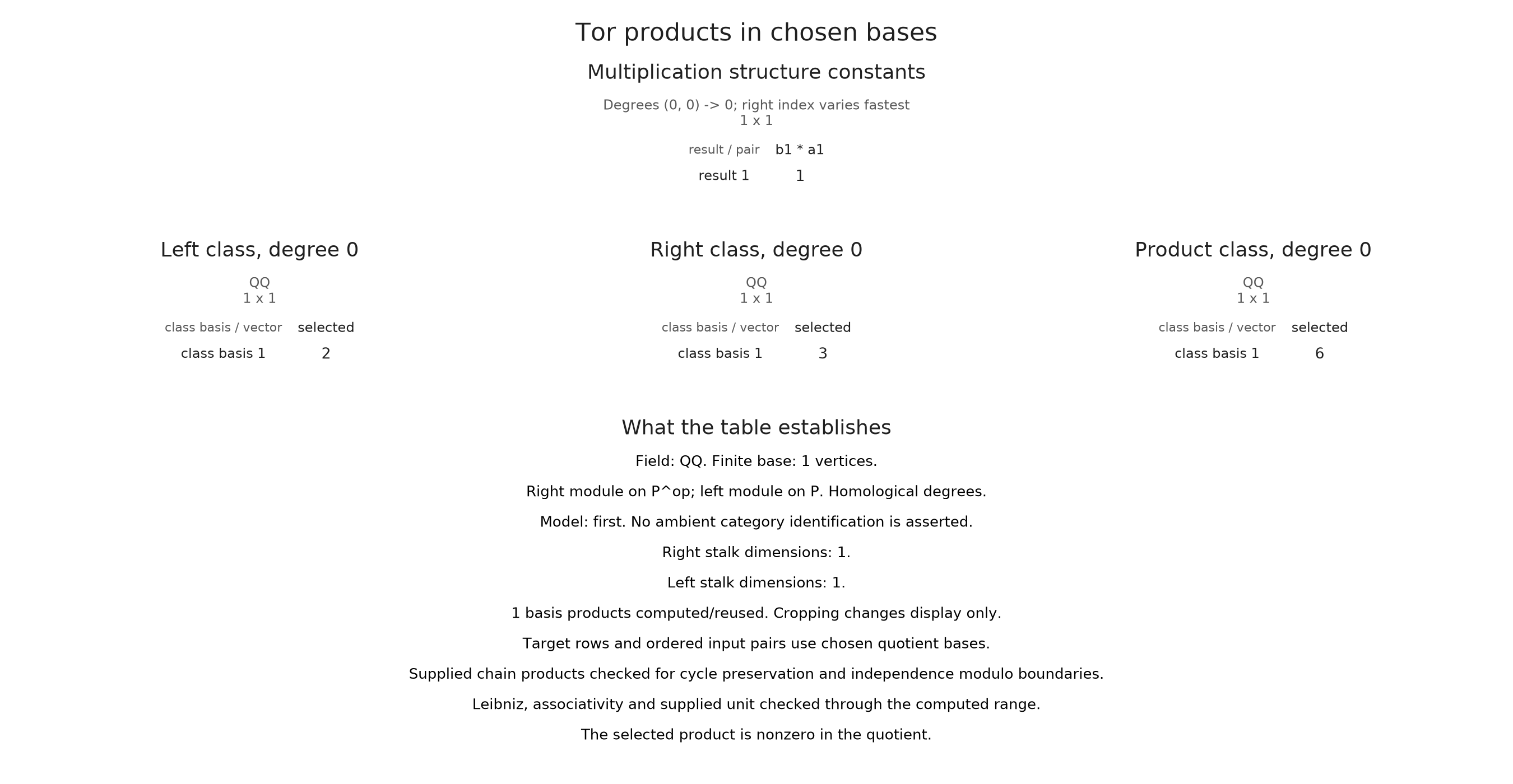
For a small example where we can state every map, take a poset with one vertex and let both modules be the field. Its tensor complex is $K$ in degree 0. We supply ordinary scalar multiplication, whose matrix is $[1]$, together with the unit 1. The selected inputs 2 and 3 should then multiply to 6.
Specifying these chain maps is a mathematical choice. Every requested Tor table checks that multiplication sends cycles to cycles and is independent of the representatives modulo boundaries. With validate_algebra=true, the request also checks the Leibniz identity relating product and differential, associativity on homology, and the supplied unit in the computed range. These conditions are explained in the implementation account.
point = OP.Advanced.FinitePoset(trues(1,1))
Kpoint = OP.Advanced.PModule{OP.QQ}(point, [1], Dict{Tuple{Int,Int},Matrix{OP.QQ}}(); field)
Tpoint = OP.tor(Kpoint,Kpoint; maxdeg=0)
scalar_algebra = OP.Advanced.TorAlgebra(Tpoint;
    mu_chain=Dict((0,0)=>sparse(reshape(OP.QQ[1],1,1))), unit_coords=OP.QQ[1])
OP.visualize(scalar_algebra; kind=:product_table, left=[2], right=[3], validate_algebra=true)
Optional: export the selected computation
The prepared specification via2 can be saved without computing its product again. PNG, SVG and PDF retain the matrix labels and the stated drawing scope. The file is a static view of the selected computation.
export_directory = mktempdir()
OP.save_visual(joinpath(export_directory,"yoneda.svg"), via2)
export_directory
"/tmp/jl_sYqcQI"Optional: prepare the product comparison
The specifications via2, via3 and zero_product already retain the answers. We select the two input coordinate columns and the output coordinate column for the browser comparison. The cocycles and boundary adjustment remain in the fuller inspection above.
@assert c2 == -c3 && all(iszero, zero_product.metadata.selection.coordinates)
product_labels = ["Through vertex 2", "Through vertex 3", "Zero left factor"]
product_views = []
for (label, answer) in zip(product_labels, (via2, via3, zero_product))
    @assert answer.metadata.selection.cycle_equation.valid
    @assert answer.metadata.selection.coordinate_equation.valid
    push!(product_views, OP.compose_visuals((
        left_class=OP.visual_panel(answer; panel=1),
        right_class=OP.visual_panel(answer; panel=2),
        product=OP.visual_panel(answer; panel=3)); columns=3, title=label,
        subtitle="The left class acts after the right; the product uses the fixed basis of E14 over Q."))
end
prepared_products = NamedTuple{Tuple(Symbol.(product_labels))}(Tuple(product_views))
derived_directory = joinpath("tamerop_outputs", "derived")
mkpath(derived_directory)
OP.save_visual_session(joinpath(derived_directory, "products.html"), prepared_products;
    selected=Symbol(first(product_labels)), size=(1400,520),
    title="Compare the two Yoneda products",
    caption="Both routes run from S1 to S4 and land in the same degree 2 Ext basis. Their rational coordinates have opposite signs; replacing the left class by zero gives zero.");
The product calculation leaves us with a concrete cocycle and its quotient class. To follow how representatives change under a map, or how a boundary adjustment explains equality of classes, continue with the complex guide. The derived reference gives the exact input and output conventions, and the implementation account develops the comparison lifts that make composition possible.