Computing interval multiplicities and splittings
Download the executed notebook · Build and environment record
Suppose we know a module's spaces and maps and want to recover simpler pieces from them. An interval supported on a few vertices is one possible piece, but it belongs to a direct sum decomposition only if we can both include it and project back onto it. We will construct a square module whose pieces we know in advance, recover their multiplicities, and inspect the maps that separate them. A second example will help us understand what can remain after an interval search.
You need TamerOp and CairoMakie, and familiarity with matrices and finite modules. The mathematical lesson develops the splitting condition; the API reference gives the call contracts. We work over the rational field on a specified finite poset, beginning with a directly supplied diagram.
import TamerOp as OP
using CairoMakie
A = OP.Advanced
QQ = Rational{BigInt}
field = OP.CoreModules.QQField();
Start with pieces we can recognize
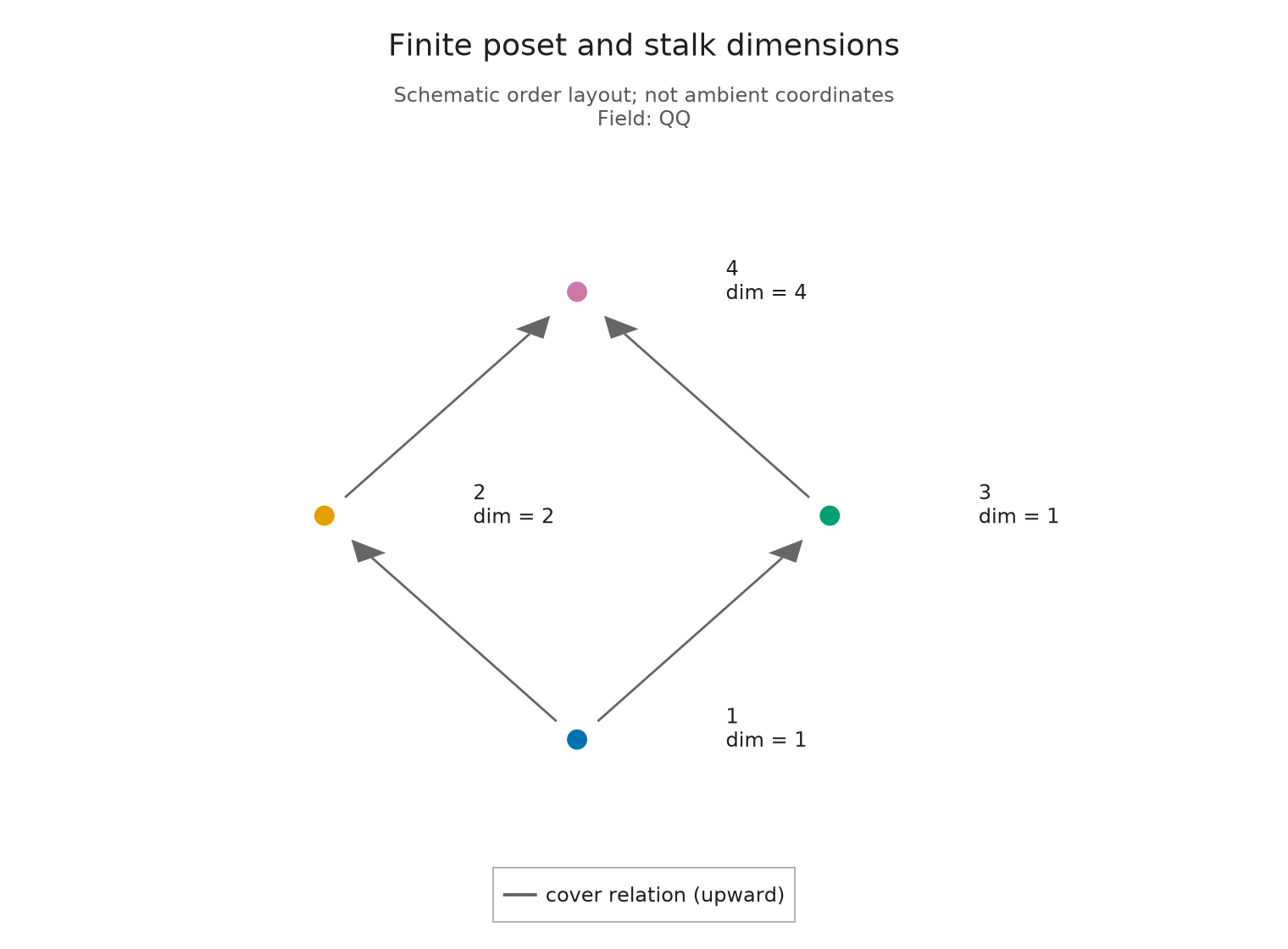
The square has vertex 1 at the bottom, vertices 2 and 3 in the middle, and vertex 4 at the top. Put one interval on the full square, one on the edge {2,4}, and two copies at vertex 4 alone. Their sum has dimensions (1,2,1,4): for instance, all four copies contribute a coordinate at the top, while only the full square reaches the bottom.
In the construction below, active[v] lists the copies present at vertex v. A cover map retains a coordinate exactly when the same copy is present at both endpoints. These coordinates reveal the answer before we run the decomposition; an independently supplied module may have bases that mix the same pieces.
P = A.ProductOfChainsPoset((2, 2))
supports = [[1, 2, 3, 4], [2, 4], [4], [4]]
active = [findall(I -> v in I, supports) for v in 1:4]
maps = Dict((u, v) => QQ[i == j for i in active[v], j in active[u]]
            for (u, v) in A.cover_edges(P))
M = A.PModule{QQ}(P, length.(active), maps; field)
@assert OP.dimensions(M).stalks == [1, 2, 1, 4]
OP.visualize(M)
Ask for one multiplicity
At vertex 4, two coordinates belong to intervals supported at that vertex alone. The other two arrive from below. We therefore expect interval_multiplicity to return 2 for {4}, since projection onto a copy supported only there must annihilate every incoming image. Restricting the module to {4} discards those incoming maps, so its generalized rank is the full stalk dimension, 4.
multiplicity = OP.interval_multiplicity(M; vertices=[4])
restricted_rank = OP.generalized_rank(M; vertices=[4])
@assert multiplicity == 2
@assert restricted_rank == 4
(; multiplicity, restricted_rank)
(multiplicity = 2, restricted_rank = 4)Choose the scope of the search
We can ask about a supplied family of intervals or let the algorithm search for all interval summands. Removing the two copies on {4} leaves dimensions (1,2,1,2), which may still contain intervals we never asked about. For this supplied family, missing records that the complete decomposability question remains unanswered.
The default search considers every support that can occur, eliminating impossible candidates from the maps at their endpoints. On our square it recovers all three interval types and leaves zero residual. By default the result retains multiplicities and residual dimensions; we will request the splitting maps separately.
selected = OP.interval_decomposition(M; family=[[4]])
@assert ismissing(OP.is_interval_decomposable(selected))
@assert A.residual_dimensions(selected) == [1, 2, 1, 2]
whole = OP.interval_decomposition(M)
@assert A.interval_family(whole) == [[1, 2, 3, 4], [2, 4], [4]]
@assert A.interval_multiplicities(whole) == [1, 1, 2]
@assert OP.is_interval_decomposable(whole) === true
OP.describe(whole)
(kind = :interval_decomposition, category = :finite_poset_representations, field = TamerOp.CoreModules.CoeffFields.QQField(), vertices = 4, interval_types = 3, interval_copies = 4, residual_dimension = 0, exhaustive = true, interval_decomposable = true, witnesses = false, search = (scanned = 3, candidates = 3, tested = 3))Recover a splitting in the supplied coordinates
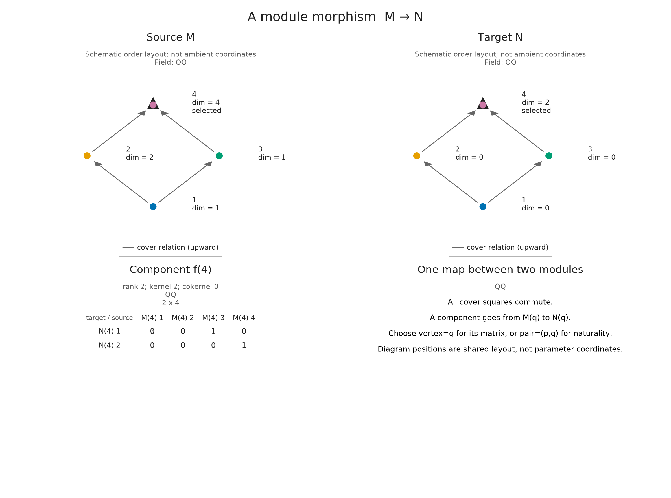
Set witnesses=true when the question needs actual modules and maps. The returned inclusion inserts the extracted interval copies into the original module, and projection takes a vector back to its component in those copies. For our two copies on {4}, the projection at vertex 4 has four input coordinates and two output coordinates. The other interval types form the residual, whose dimensions are still (1,2,1,2).
split = OP.interval_decomposition(M; family=[[4]], witnesses=true)
w = A.decomposition_maps(split)
@assert A.check_interval_decomposition(split; throw=true).splitting_checked
@assert OP.dimensions(w.summand).stalks == [0, 0, 0, 2]
@assert OP.dimensions(w.residual).stalks == [1, 2, 1, 2]
OP.visualize(w.projection; vertex=4)
The inclusions and projections let us check how a vector is recovered. Write $i,p$ for the interval inclusion and projection, and $j,q$ for the residual pair. The composites $ip$ and $jq$ are projections onto the two components inside $M$. They satisfy $ip+jq=1_M$ at every vertex, so adding those components returns the original vector.
The loop below checks this reconstruction in the supplied bases. The preceding validator also checks that the maps commute with the module's arrows, that $pi$ and $qj$ are identities, and that the mixed composites $pj$ and $qi$ vanish. These conditions make the separate decompositions of the stalks agree across the diagram.
using LinearAlgebra
for v in 1:4
    i = A.component(w.inclusion, v)
    p = A.component(w.projection, v)
    j = A.component(w.residual_inclusion, v)
    q = A.component(w.residual_projection, v)
    @assert i * p + j * q == Matrix{QQ}(LinearAlgebra.I, OP.dimensions(M, v).stalk, OP.dimensions(M, v).stalk)
end
OP.describe(split)
(kind = :interval_decomposition, category = :finite_poset_representations, field = TamerOp.CoreModules.CoeffFields.QQField(), vertices = 4, interval_types = 1, interval_copies = 2, residual_dimension = 6, exhaustive = false, interval_decomposable = missing, witnesses = true, search = (scanned = 1, candidates = 1, tested = 1))See a residual that contains no intervals
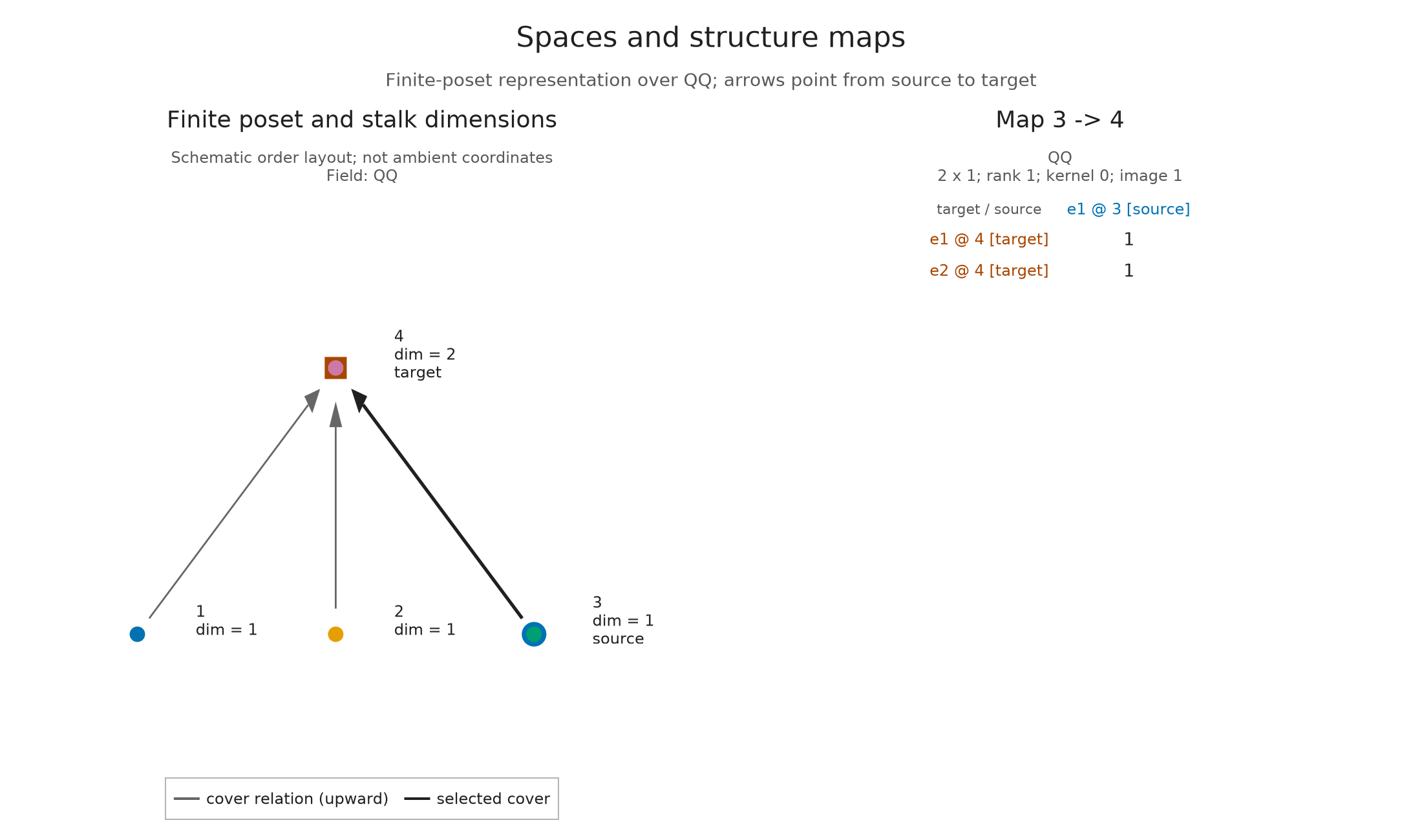
Now let three incomparable source spaces map into a common sink $k^2$, with image lines spanned by $(1,0)$, $(0,1)$ and $(1,1)$. Any two lines span the sink. A projection onto an interval carrying just one source would have to vanish on the other two lines and hence vanish everywhere, so it could not retract onto the chosen line. An interval carrying several sources would require their images to lie in a single line. The lesson's diagram and argument cover the remaining possible supports.
A complete interval search should therefore leave the entire module. We display the map from source 3 to the sink alongside that result, so the column $(1,1)$ remains visible.
star = A.FinitePoset(Bool[1 0 0 1; 0 1 0 1; 0 0 1 1; 0 0 0 1])
three_lines = A.PModule{QQ}(star, [1, 1, 1, 2],
    Dict((1, 4) => reshape(QQ[1, 0], 2, 1),
         (2, 4) => reshape(QQ[0, 1], 2, 1),
         (3, 4) => reshape(QQ[1, 1], 2, 1)); field)
remainder = OP.interval_decomposition(three_lines; witnesses=true)
@assert OP.is_interval_decomposable(remainder) === false
@assert isempty(A.interval_multiplicities(remainder))
@assert A.residual_dimensions(remainder) == [1, 1, 1, 2]
OP.visualize(A.decomposition_maps(remainder).residual; kind=:module_inspector, pair=(3, 4))
Use the same algebra after encoding
An EncodingResult retains the finite module together with the map assigning original parameters to finite labels. The interval query still refers to those labels: {4} means vertex 4 of the encoding poset. A splitting on that poset pulls back along the encoding map, but completeness in a different category requires its own hypotheses. The result's provenance records which finite category the calculation used.
For repeated queries on an encoded input, a SessionCache can reuse its materialized finite module. Here that module is already supplied, so we can compare the answers directly with the earlier calls.
classifier = A.GridEncodingMap(P, ([0, 1], [0, 1]))
encoded = OP.EncodingResult(P, M, classifier)
cache = OP.SessionCache()
@assert OP.interval_multiplicity(encoded; vertices=[4], cache) == 2
encoded_result = OP.interval_decomposition(encoded; cache)
@assert OP.is_interval_decomposable(encoded_result) === true
OP.provenance(encoded_result)
(category = :finite_poset_representations, base_poset = ProductOfChainsPoset(axes=(2, 2), orientation=(1, 1), nvertices=4), field = TamerOp.CoreModules.CoeffFields.QQField(), model = :hom_composition_pairing, candidate_pruning = :top_socle_degree_zero, exhaustive = true, ambient_identification = :not_asserted)Put the pieces beside the whole module
The retained maps also let us inspect several pieces together. We request all interval witnesses and prepare a summand_session, whose snapshot can be drawn as a static figure. Its first row compares the full module, the selected blocks, and their complement; the remaining panels show the individual pieces and the selected maps.
A block groups copies of the same interval type. Thus block 3 contains both copies on {4}, contributing dimension two there. Selecting blocks 2 and 3 gives dimensions (0,1,0,3), with the constant square (1,1,1,1) left as complement. The node positions describe the finite order, and keeping them fixed across panels makes these additions visible at each vertex.
complete = OP.interval_decomposition(M; witnesses=true)
collection = OP.summand_collection(complete)
viewer = OP.summand_session(collection; selected=[2, 3], focus=3, vertex=4)
view = A.inspection_snapshot(viewer)
@assert view.metadata.selected_dimensions == [0, 1, 0, 3]
@assert view.metadata.complement_dimensions == [1, 1, 1, 1]
OP.visualize(view)
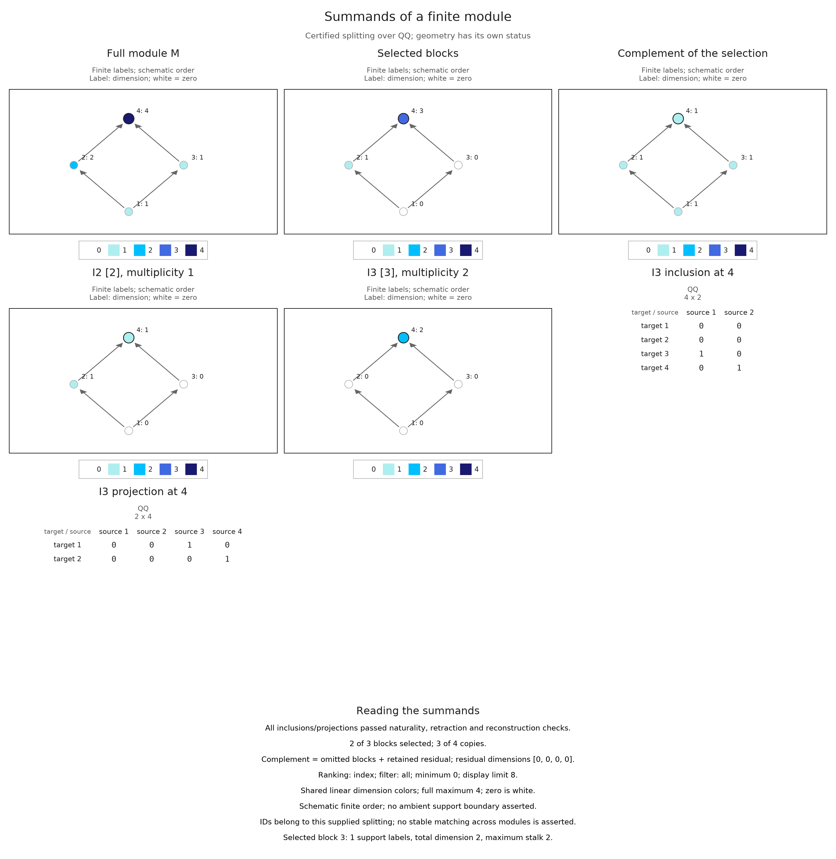
Use the prepared comparison to select the constant square, the edge, the two copies at vertex 4, or the edge together with those two copies. Follow vertex 4 across the first row: its full dimension stays four, while the selected and complementary dimensions change. The same addition holds at each vertex.
Block 3 keeps its two copies together, so selecting it contributes dimension two at the top. The detail panels retain the inclusion and projection of the focused block, supplying the maps behind these dimension counts. The choices use one fixed computed splitting; changing the selection does not search for a new decomposition.
Explore the selected summands and their complement
Recover supports in the parameter plane
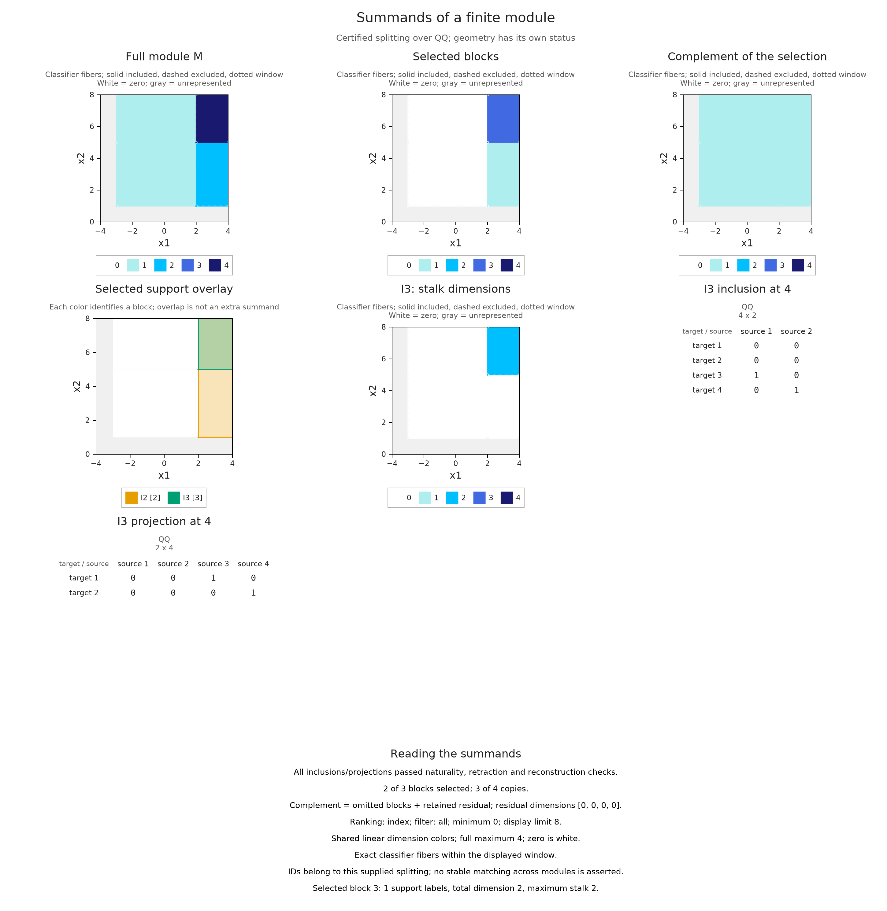
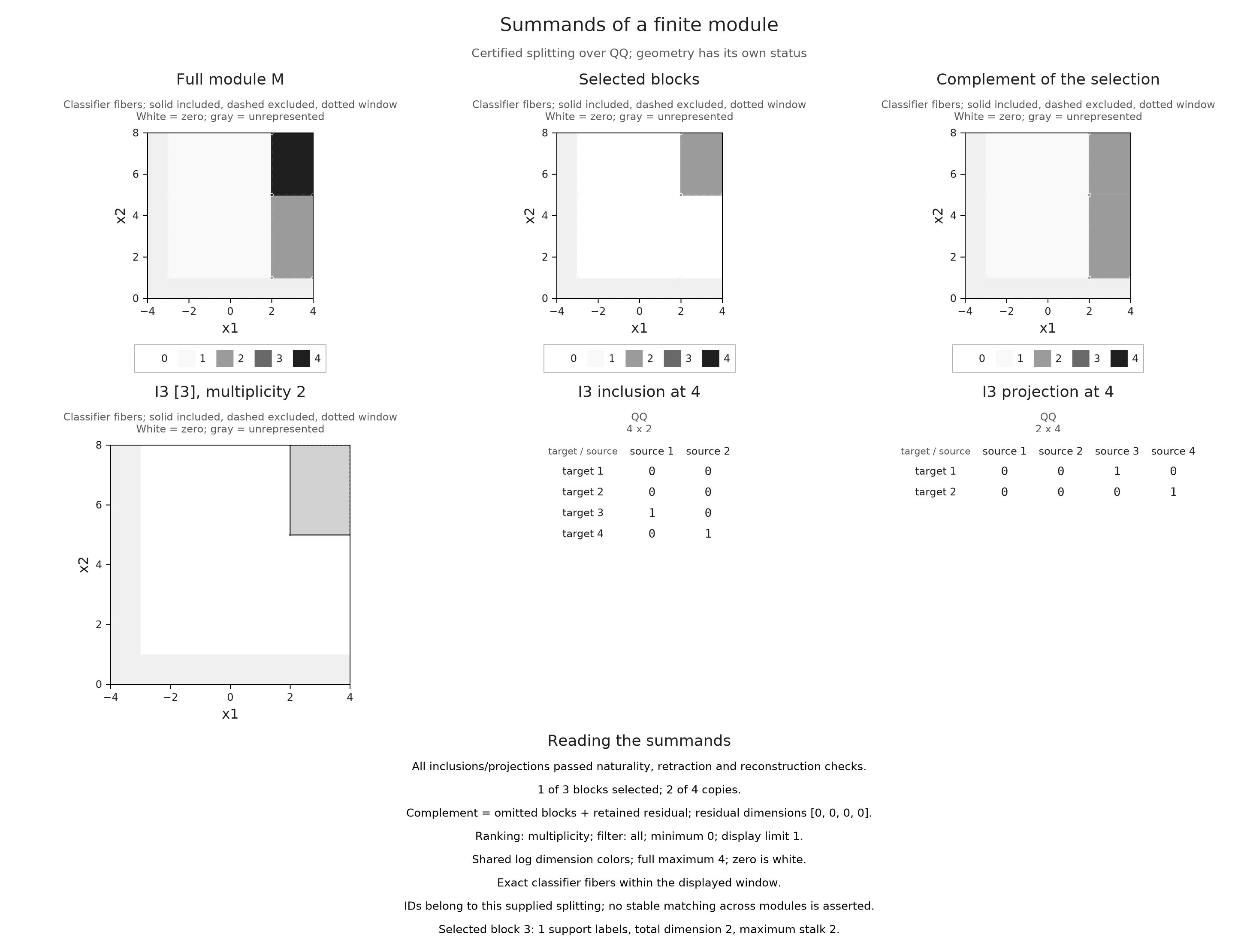
An encoding map lets us place these finite labels back in the original parameter domain. Here its thresholds are [-3,2] in the first coordinate and [1,5] in the second. Each grid cell includes its lower edge and stops just before the next threshold; cells beyond the final threshold continue indefinitely. The two copies at the top vertex therefore occupy $x\geq2$, $y\geq5$, clipped to the chosen drawing window.
The edge interval contributes one dimension throughout $x\geq2$, $y\geq1$. Where it overlaps the two top copies, their selected sum has dimension three. Solid edges are included, dashed edges excluded, and dotted edges mark the viewing window. Gray denotes a parameter with no finite label, while white denotes a represented stalk of dimension zero. These boundary conventions come from the encoding map.
support_encoding = OP.EncodingResult(P, M,
    A.GridEncodingMap(P, ([-3, 2], [1, 5])))
support_viewer = OP.summand_session(collection; encoding=support_encoding,
    box=([-4, 0], [4, 8]), selected=[2, 3], focus=3, vertex=4,
    layout=:overlay)
OP.visualize(A.inspection_snapshot(support_viewer))
Choose which blocks to compare
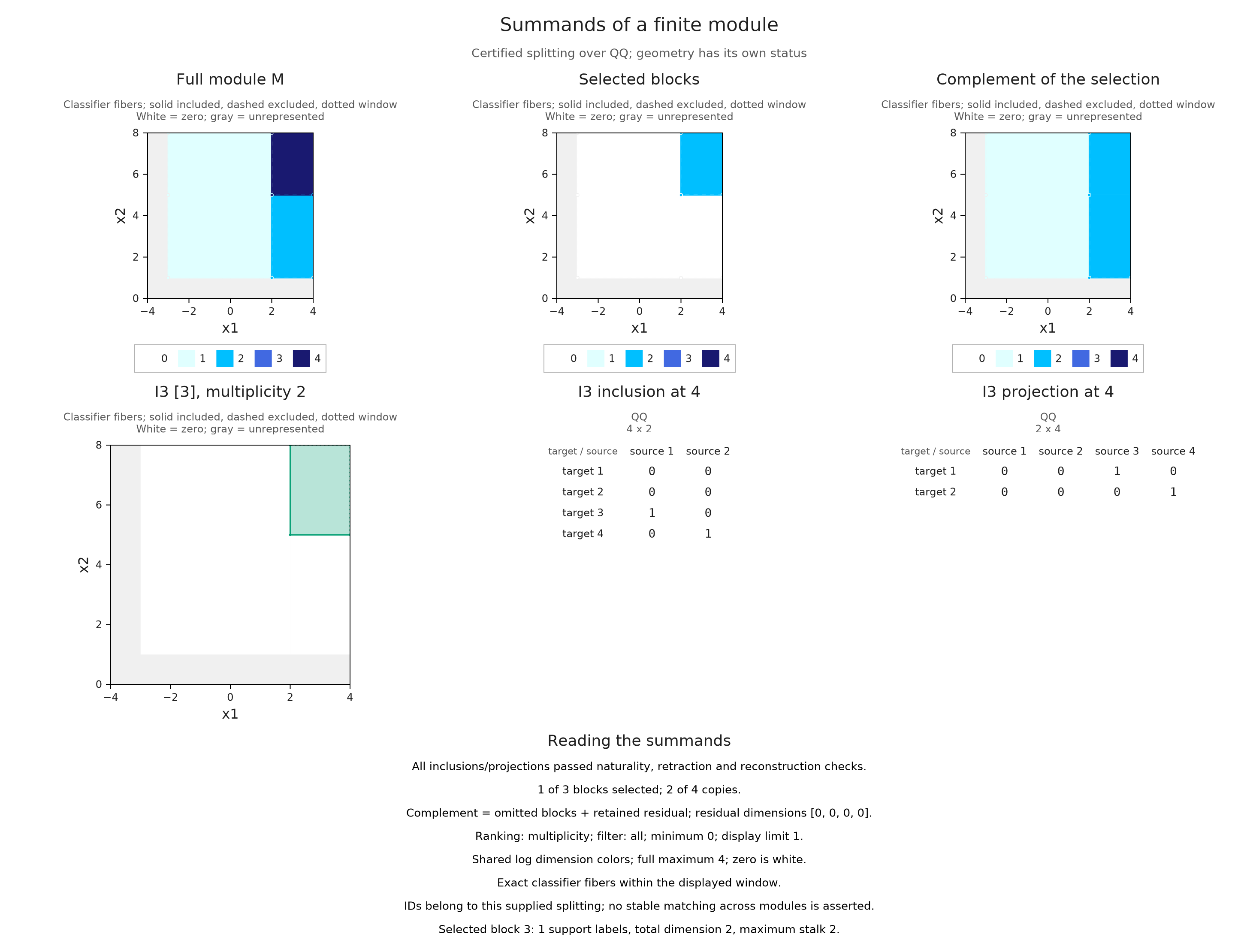
The statistic used to order a gallery should match the question we want to ask. Multiplicity counts copies of an interval, support size counts finite labels, and total dimension adds the stalk dimensions over those labels. The latter two depend on the chosen finite description and do not measure area in the parameter plane.
Here sorting by multiplicity puts block 3 first. Keeping only that block selects its two copies at vertex 4 and leaves dimensions (1,2,1,2) in the complement. The original block IDs survive sorting. We use a logarithmic color scale, which still distinguishes zero, and retain a shared scale based on the full module so that a selection change cannot silently rescale the colors.
A.select_inspection!(support_viewer; selected=nothing,
    sort_by=:multiplicity, limit=1, layout=:isolate, scale=:log)
@assert A.inspection_selection(support_viewer).ids == [3]
@assert A.inspection_snapshot(support_viewer).metadata.complement_dimensions == [1, 2, 1, 2]
OP.visualize(A.inspection_snapshot(support_viewer))
Look at maps between the pieces
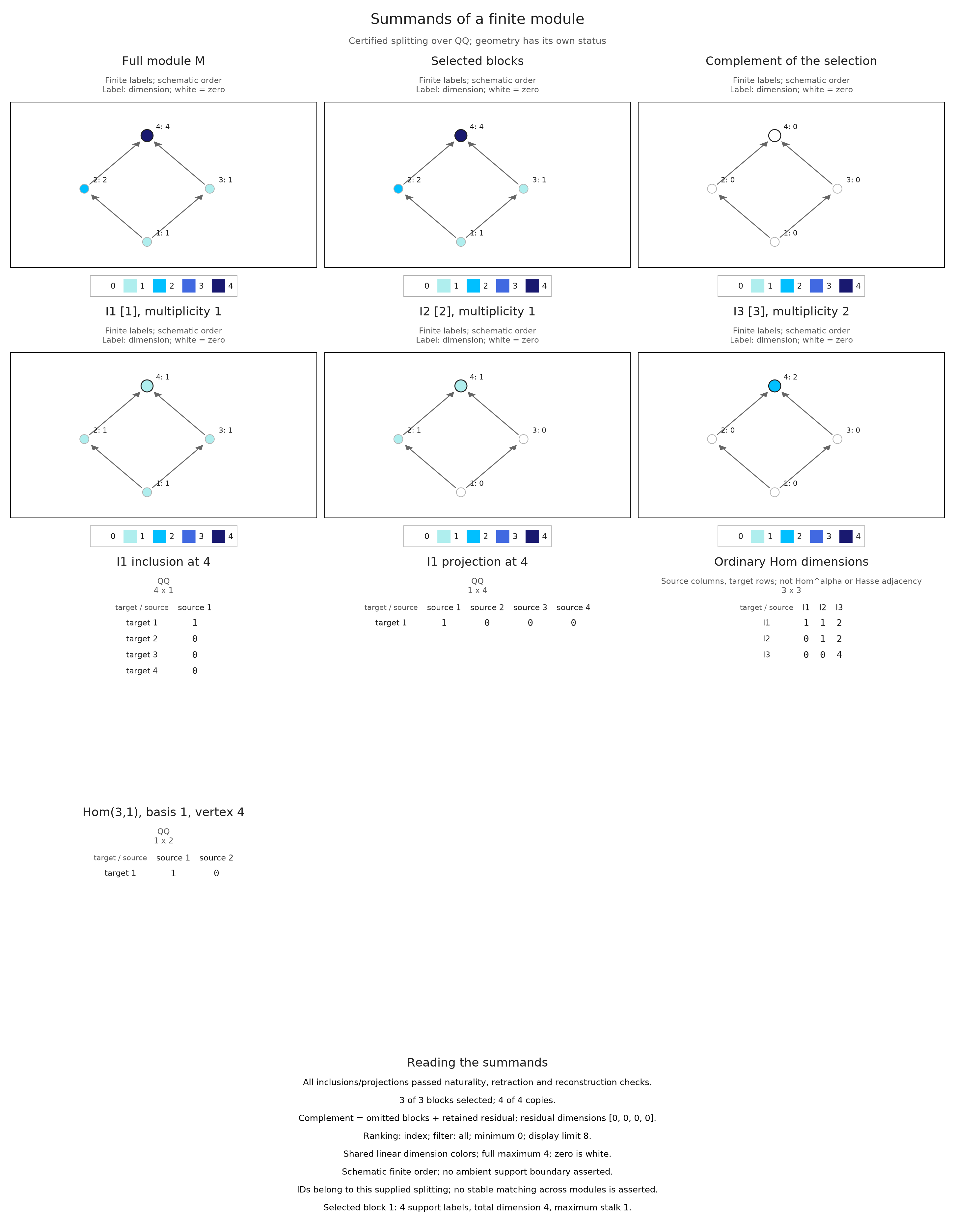
The chosen projections annihilate the other summands, but further module maps may exist between those summands. For example, a map from the two copies at vertex 4 into the constant square can choose any row at the sink, giving two independent maps. In the other direction, compatibility with an incoming arrow forces the sink component to vanish.
The Hom table records the dimensions of these spaces of module maps. Sources occupy columns and targets occupy rows. Selecting a pair then displays one basis map in the retained coordinates; for source block 3 and target block 1, its component at vertex 4 is a row with two entries. Requesting hom=true performs this additional algebra, with bounds separate from the cost of drawing the gallery.
A.select_inspection!(viewer; selected=nothing, hom=true,
    hom_pair=(3, 1), vertex=4)
hom_view = A.inspection_snapshot(viewer)
@assert hom_view.metadata.hom_dimensions == [1 1 2; 0 1 2; 0 0 4]
@assert size(hom_view.metadata.hom_component) == (1, 2)
OP.visualize(hom_view)
Inspect a supplied piece with thicker stalks
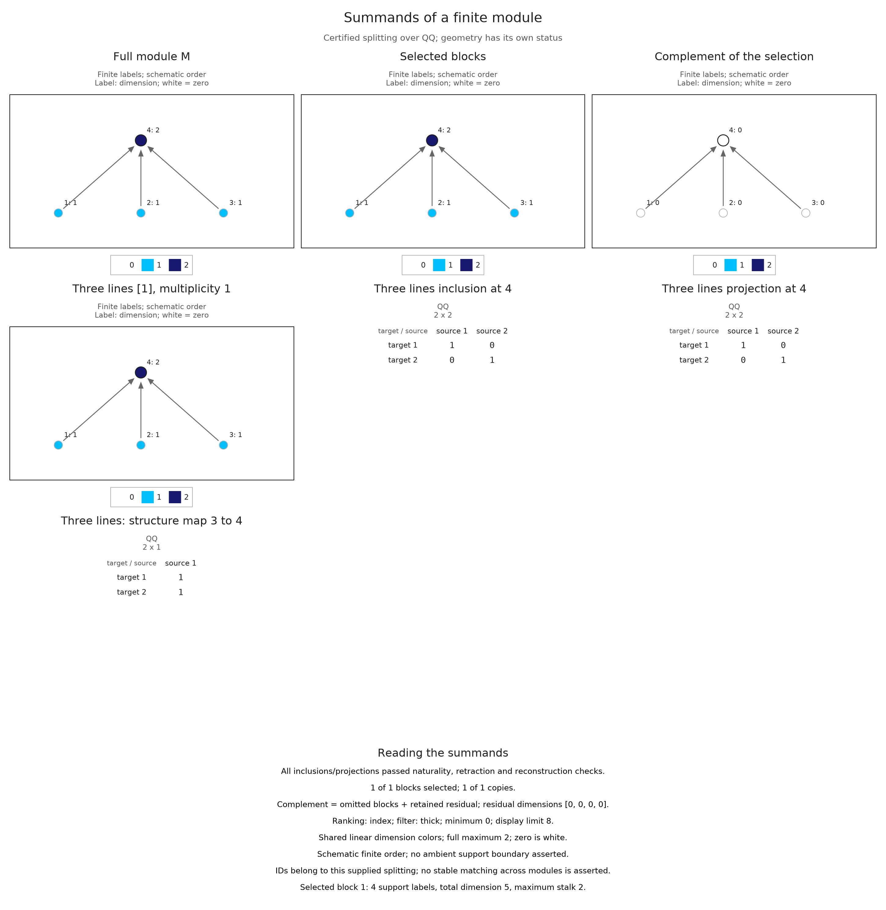
We can inspect a supplied splitting without recomputing how its pieces were found. To see what the viewer checks, regard the three-line module above as one piece of itself and supply the identity in both directions. These maps certify a summand; the adapter does not test whether that summand is indecomposable. TamerOp's separate indecomposable_decomposition operation addresses that algebraic question.
This piece has three stalks of dimension one and a sink of dimension two. Selecting the third arrow recovers the column $(1,1)$. Its dimension panel shows what a uniform support fill would omit: the space changes size within the connected support.
identity_map = OP.Modules.id_morphism(three_lines)
thick = OP.summand_collection(three_lines, [three_lines];
    inclusions=[identity_map], projections=[identity_map], labels=["Three lines"])
OP.visualize(thick; type_filter=:thick, pair=(3, 4), vertex=4)
With WGLMakie loaded, OP.visualize(viewer; backend=:wglmakie) opens the retained data in a live inspector. The labelled controls select block IDs, filters and maps; clicking a node or an encoding cell selects its finite label. Invalid entries leave the previous selection in place, and hover reads already prepared data. Live selection requires Julia to remain running. The session guide explains the supported display paths.
A support drawing supplied independently of the encoding needs a separate interpretation. A.SummandSupportDrawing accepts unions of half-open boxes together with their provenance and a stated error claim. The viewer labels that geometry as unverified because it checks the splitting maps, not the asserted geometric accuracy. Signed summaries and tracks obtained by matching sampled slices likewise retain their own meanings.
Bound a search deliberately
The number of candidate intervals can grow exponentially with the finite poset. A supplied family is useful when those particular supports are the question; for a complete search, choose budgets that fit the intended input. Reaching a budget raises an error before returning a result. It therefore cannot be mistaken for a proof that the module fails to split.
The calls here use exact rational arithmetic. Prime fields are supported as well; approximate splittings with floating coefficients require different criteria. The small budget below is sufficient for our square, and interval_candidates shows which supports survive the preliminary endpoint tests.
budget = A.IntervalDecompositionBudget(max_vertices=4, max_dimension=16,
    max_matrix_entries=1000, max_antichains=16, max_candidates=256)
@assert OP.is_interval_decomposable(M; budget) === true
A.interval_candidates(M; budget)
3-element Vector{Vector{Int64}}:
 [1, 2, 3, 4]
 [2, 4]
 [4]
Optional: change the view without changing the answer
A palette can help distinguish support regions when preparing a figure for another setting. Here the grayscale palette changes both the support colors and the shared dimension scale. The retained multiplicities, splitting maps and boundary conventions are unchanged.
style = OP.VisualStyle(palette=:grayscale)
OP.visualize(A.inspection_snapshot(support_viewer); style)
Prepare the summand comparisons
Optional: Prepare the summand comparisons
Each choice below selects blocks from the same checked collection. We verify their dimensions against the supplied supports, then check that the complementary dimensions recover the full module at every vertex. Saving these snapshots retains the displayed maps and the selections used by the comparison.
prepared_summands = OP.summand_session(collection; selected=[1], focus=1, vertex=4)
summand_views = Pair{Symbol,Any}[]
choices = (("Constant square", [1], [1,1,1,1]),
           ("Edge {2,4}", [2], [0,1,0,1]),
           ("Two copies at {4}", [3], [0,0,0,2]),
           ("Edge and two top copies", [2,3], [0,1,0,3]))
for (name, ids, expected_dimensions) in choices
    A.select_inspection!(prepared_summands; selected=ids, focus=last(ids), vertex=4)
    snapshot = A.inspection_snapshot(prepared_summands)
    @assert snapshot.metadata.selected_dimensions == expected_dimensions
    @assert snapshot.metadata.selected_dimensions + snapshot.metadata.complement_dimensions == [1,2,1,4]
    focus_panel = 3 + findfirst(==(last(ids)), ids)
    inclusion_panel = length(snapshot.panels) - 2
    projection_panel = length(snapshot.panels) - 1
    picture = OP.compose_visuals((
        full=OP.visual_panel(snapshot; panel=1),
        selected=OP.visual_panel(snapshot; panel=2),
        complement=OP.visual_panel(snapshot; panel=3),
        focus=OP.visual_panel(snapshot; panel=focus_panel),
        inclusion=OP.visual_panel(snapshot; panel=inclusion_panel),
        projection=OP.visual_panel(snapshot; panel=projection_panel));
        columns=3, title=name,
        subtitle="Rational coefficients; full dimensions = selected dimensions + complement dimensions")
    push!(summand_views, Symbol(name) => picture)
end
mkpath(joinpath("tamerop_outputs", "summands"))
OP.save_visual_session(joinpath("tamerop_outputs", "summands", "selected_blocks.html"),
    (; summand_views...); selected=Symbol("Edge and two top copies"),
    title="Separate summands and recover their complement",
    caption="Choose blocks of the rational square module. Their dimensions and those of the complement add to (1,2,1,4). Block 3 contains two copies at vertex 4. All views use the same computed inclusion and projection maps. Node positions describe the finite order, and colors use one shared dimension scale.", size=(1450,900))
A.close_inspection!(prepared_summands);
A.close_inspection!(viewer)
A.close_inspection!(support_viewer);
Continue with the algorithm
The implementation account explains why composing maps into and out of an interval recovers its multiplicity, then shows how endpoint information makes a complete search possible. To ask instead about persistence through a restricted region, continue with generalized ranks.