Querying regions and building GRIL features
Download the executed notebook · Build and environment record
A finite encoding retains the maps between its vector spaces. When a region branches, these maps let us ask whether vectors arriving along different branches agree. We will start with two lines mapping into a plane, then follow the same question through a signed region summary and a barcode along a grid boundary. Finally, we will let a geometric region expand and measure how wide it can become while retaining a chosen rank. These widths form the generalized rank invariant landscape, abbreviated GRIL.
Use TamerOp and CairoMakie, with some familiarity with matrices and finite modules. Our examples begin directly with vector spaces and maps over the rational numbers. OP.Advanced, abbreviated A below, supplies their constructors and the operations for inspecting a computation. The implementation account explains the matrices behind the ranks; the reference specifies the available selections.
import TamerOp as OP
using CairoMakie
const A = OP.Advanced
const QQ = Rational{BigInt}
field = OP.CoreModules.QQField();
Follow both branches into the same plane
Vertices 1 and 2 each carry a line, and their common target 3 carries a plane. In parallel, both arrows send the vector 1 to the first coordinate vector of the plane. In transverse, the second arrow sends it to the second coordinate vector. Every arrow has rank one in both modules, but the image lines intersect differently.
A compatible choice of vectors must agree after following either arrow. The generalized rank measures the image of these compatible choices after vectors related by the maps are identified. For this particular fork, the target plane already supplies that common space, so the answer is the dimension of the intersection of the two image lines. We therefore expect ranks one and zero.
fork = A.FinitePoset(Bool[1 0 1; 0 1 1; 0 0 1])
parallel = A.PModule{QQ}(fork, [1, 1, 2],
    Dict((1, 3) => reshape(QQ[1, 0], 2, 1),
         (2, 3) => reshape(QQ[1, 0], 2, 1)); field)
transverse = A.PModule{QQ}(fork, [1, 1, 2],
    Dict((1, 3) => reshape(QQ[1, 0], 2, 1),
         (2, 3) => reshape(QQ[0, 1], 2, 1)); field)
@assert Dict(OP.rank_invariant(parallel)) == Dict(OP.rank_invariant(transverse))
ranks = (OP.generalized_rank(parallel; vertices=1:3),
         OP.generalized_rank(transverse; vertices=1:3))
@assert ranks == (1, 0)
ranks
(1, 0)OP.visualize(parallel; kind=:generalized_rank, vertices=1:3)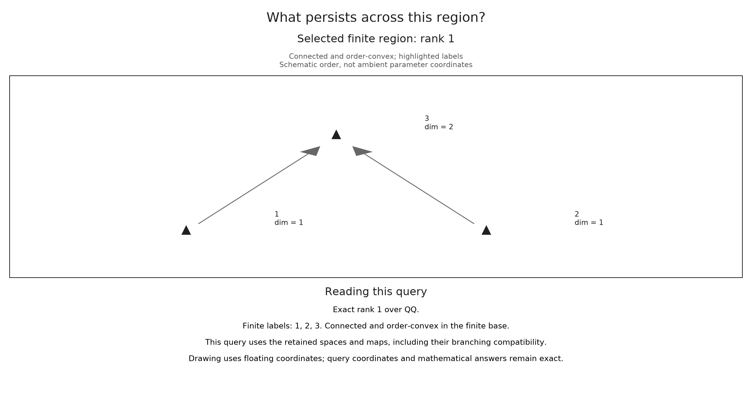
The highlighted labels specify the query. This is a drawing of the order relations, so horizontal distances between vertices have no parameter units. In transverse, the two image lines meet only at zero even though the stalk dimensions and the ranks of individual maps agree with parallel.
The query must be nonempty, connected by comparabilities, and order convex: whenever it contains the ends of an order interval, it must contain every label between them. The set [1,2] is disconnected because those two vertices are incomparable. check_generalized_rank_region detects this before computing any matrices.
@assert !A.check_generalized_rank_region(parallel; vertices=[1, 2]).valid
session = OP.generalized_rank_session(parallel; vertices=1:3)
A.select_inspection!(session; witnesses=true)
@assert A.inspection_summary(session).rank == 1
OP.visualize(A.inspection_snapshot(session))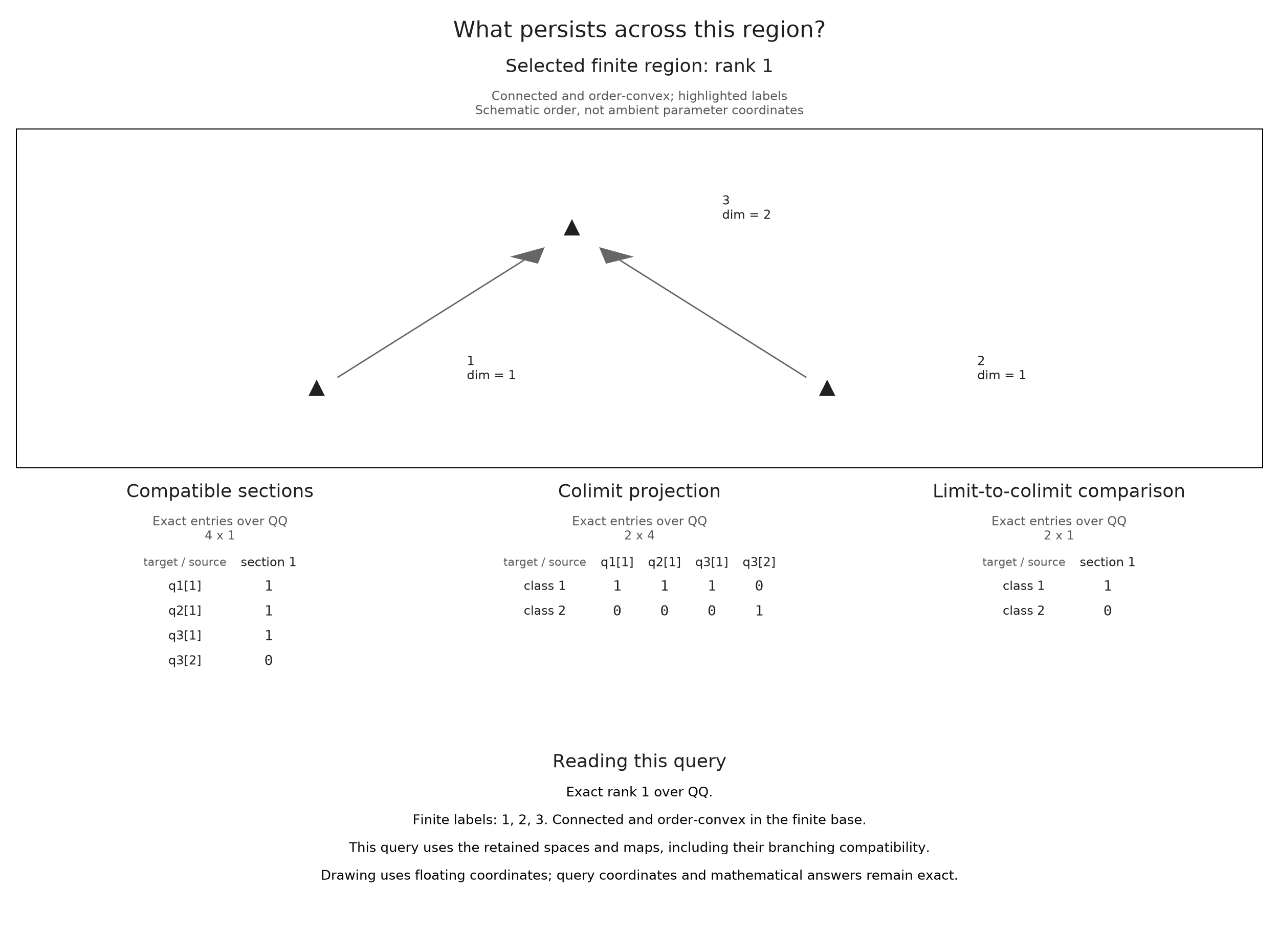
Requesting witnesses=true retains the matrices behind the scalar answer. The limit basis records compatible vectors, and the colimit projection identifies vectors related by the maps; their comparison matrix has one independent column in this example. Rows and columns use the displayed coordinates, whose bases need not be canonical.
To separate a branch from the whole region, select only vertices 2 and 3 in transverse. Its rank should still be one: the lack of a common vector across both branches does not make either arrow zero.
@assert OP.generalized_rank(transverse; vertices=[2, 3]) == 1
A.close_inspection!(session);
The prepared comparison lets you switch between the two complete forks and the second branch of transverse. Keep the target plane in mind as the highlighted region changes. Coincident image lines give rank one on the whole fork. Different image lines give rank zero there, while the single branch still has rank one. The displayed matrices express compatible vectors and their common images in the coordinates of each query.
Compare the fork and its second branch
Reconstruct ranks on a declared family
Give the plane a third incoming line, then query the target and each branch separately. Each branch has rank one and the target has dimension two. If we add the three branch contributions at their common target, we get three; a coefficient of −1 on the target corrects this to two. This is a signed reconstruction of four rank queries, so the negative coefficient has no interpretation as a negative dimension of a summand.
star = A.FinitePoset(Bool[1 0 0 1; 0 1 0 1; 0 0 1 1; 0 0 0 1])
three_lines = A.PModule{QQ}(star, [1, 1, 1, 2],
    Dict((1, 4) => reshape(QQ[1, 0], 2, 1),
         (2, 4) => reshape(QQ[0, 1], 2, 1),
         (3, 4) => reshape(QQ[1, 1], 2, 1)); field)
signed = OP.interval_rank_summary(three_lines; family=[[4], [1, 4], [2, 4], [3, 4]])
@assert A.interval_coefficients(signed) == [-1, 1, 1, 1]
@assert A.reconstruct_rank(signed; vertices=[4]) == 2
OP.visualize(signed; query=(vertices=[4],))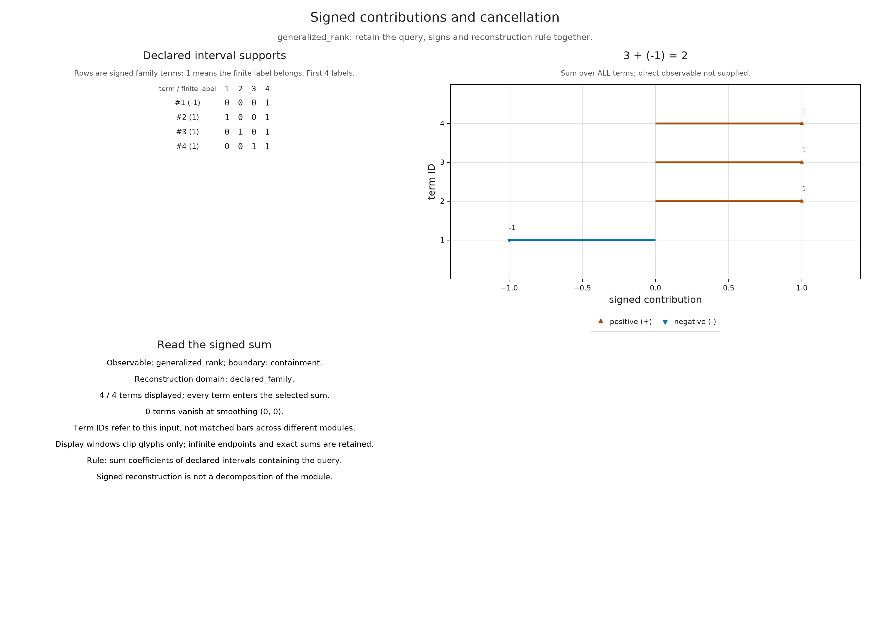
The reconstruction holds on the four regions supplied in family. For another region, compute a new rank query: this table need not determine it. The signed contributions guide explains how to inspect the contribution of each term.
Read a grid region through its boundary zigzag
On a grid we can describe a region using a path around its boundary. A zigzag is a sequence of spaces with an arrow between consecutive positions, where each arrow may point forward or backward. Its bars record consecutive positions across which a class persists. For the boundary path used here, bars extending across the whole path count the generalized rank of the region.
Start with a grid of nine labels in product order, numbered with the first coordinate varying fastest. We specify three interval summands: one on the entire grid, one on the lower right square and one on the upper left square. At each label we keep a coordinate for every active summand, and the maps preserve the coordinates that continue. The query 2:8 omits two opposite corners. Only the summand on the entire grid covers it, so its rank should be one. Unequal axis spacings keep physical parameter coordinates distinguishable from grid indices.
grid_poset = A.ProductOfChainsPoset((3, 3))
supports = [collect(1:9), [2, 3, 5, 6], [4, 5, 7, 8]]
active = [findall(s -> q in s, supports) for q in 1:9]
grid_maps = Dict((a, b) => QQ[i == j for i in active[b], j in active[a]]
                for (a, b) in A.cover_edges(grid_poset))
grid_module = A.PModule{QQ}(grid_poset, length.(active), grid_maps; field)
grid = A.GridEncodingMap(grid_poset, ([0, 2, 4], [0, 3, 6]))
encoded = OP.EncodingResult(grid_poset, grid_module, grid)
boundary_session = OP.generalized_rank_session(encoded; vertices=2:8, boundary=true)
@assert A.inspection_summary(boundary_session).rank == 1
OP.visualize(A.inspection_snapshot(boundary_session))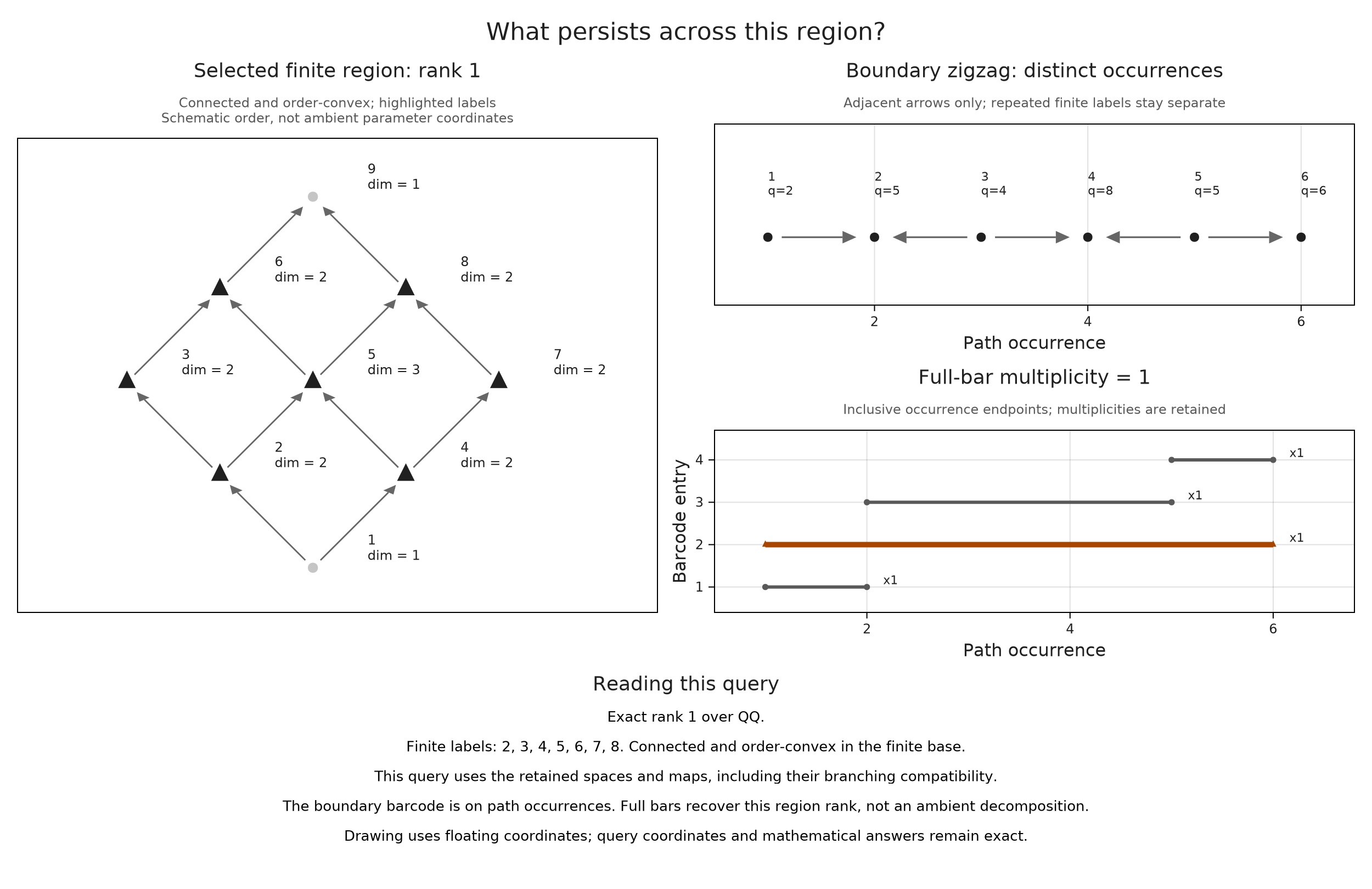
The boundary path visits labels 2,5,4,8,5,6. Its two visits to label 5 are separate positions, with arrows only between consecutive positions and the maps obtained by composing those arrows. Adding every order relation among the underlying grid labels would change this diagram. Bars use occurrence indices and include both endpoints; the full bar covers all six positions and has multiplicity one.
The boundary cap theorem applies to connected convex intervals in the two dimensional index lattice. The resulting bars describe the path restriction, rather than an interval decomposition of the ambient module. The algorithm account explains which boundary path the theorem requires and how its computation is bounded.
boundary = A.boundary_zigzag(grid_module, grid; vertices=2:8)
@assert A.boundary_path(boundary).vertices == [2, 5, 4, 8, 5, 6]
@assert OP.generalized_rank(boundary) == 1
A.select_inspection!(boundary_session; occurrence=5)
OP.describe(boundary)
(kind = :boundary_zigzag, rank = 1, occurrences = 6, distinct_labels = 5, intervals = 4, queries = 22, interpretation = :finite_grid_interval, field = TamerOp.CoreModules.CoeffFields.QQField())Move from finite labels to a continuous worm
For a geometric region, we must specify how the finite labels represent the parameter plane. Consider a one dimensional space at every point of the quadrant $[0,\infty)^2$, with identity maps there and zero spaces elsewhere. One grid label encodes it. The grid convention extends values constantly to the upper and right tails and assigns zero below either first coordinate.
A worm centered at $p=(p_x,p_y)$, with width $d\geq0$ and integer length $\ell\geq1$, is the closed region defined by
\[|x-p_x|\leq\ell d,\quad |y-p_y|\leq\ell d,\quad |x+y-p_x-p_y|\leq2d.\]
At length one these inequalities describe a square. Larger lengths stretch it along the anti-diagonal while the last inequality cuts off two opposite corners. Every point satisfying the inequalities belongs to the query; sampling a few squares would give a different region.
one_label = A.ProductOfChainsPoset((1, 1))
quadrant_module = A.PModule{QQ}(one_label, [1],
    Dict{Tuple{Int,Int},Matrix{QQ}}(); field)
quadrant_grid = A.GridEncodingMap(one_label, ([0], [0]))
quadrant = OP.EncodingResult(one_label, quadrant_module, quadrant_grid)
worm_session = OP.generalized_rank_session(quadrant; center=(4, 6), width=2, length=2,
    levels=(1, 2), lengths=(1, 2, 4))
@assert A.inspection_summary(worm_session).rank == 1
OP.visualize(A.inspection_snapshot(worm_session))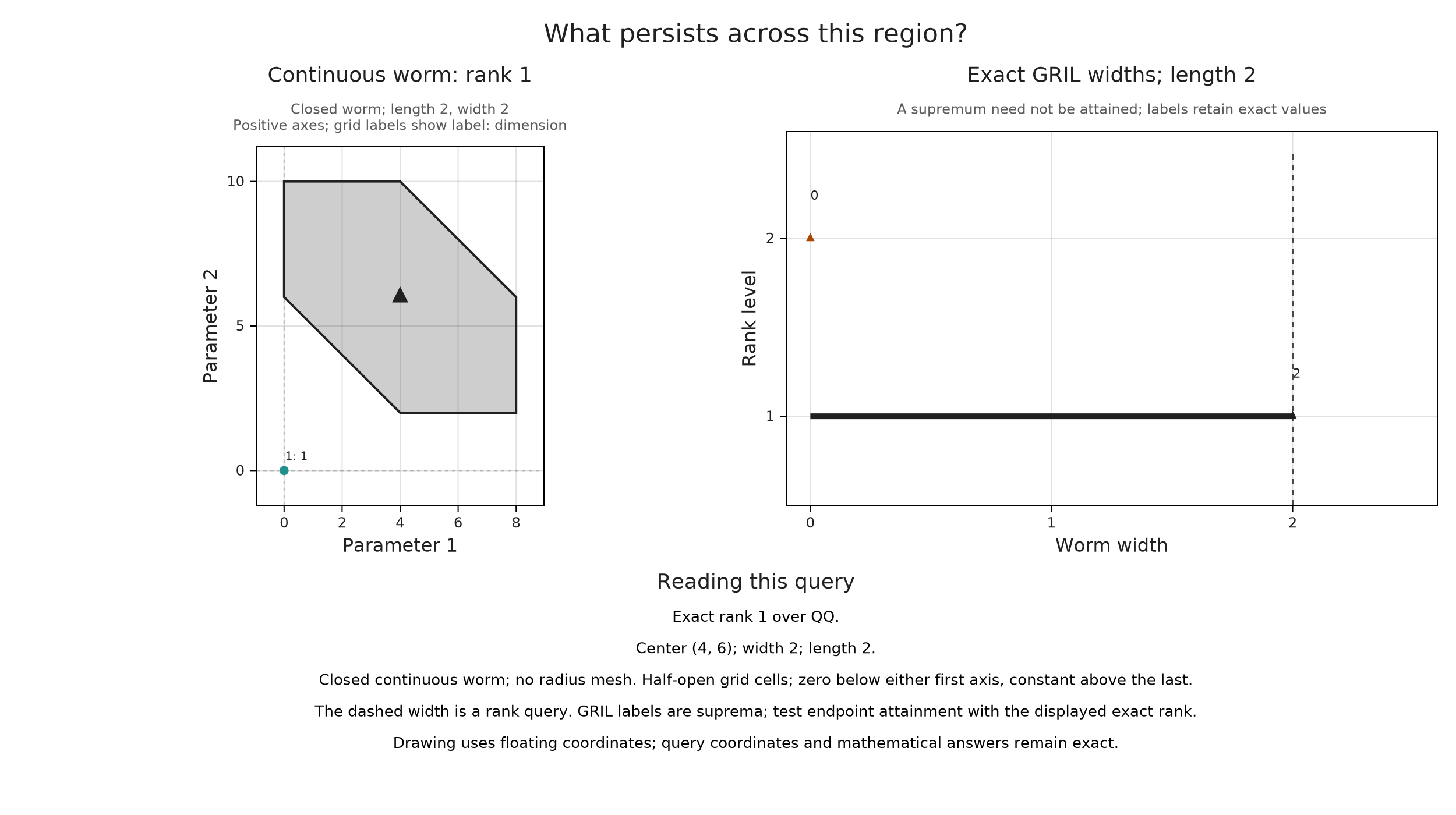
For each rank level $k$, GRIL gives the supremum of widths whose generalized rank is at least $k$. Here a worm of length $\ell$ remains inside the quadrant while its width is at most $4/\ell$: the center's first coordinate, four, reaches its boundary before the second coordinate, six. The level one widths for lengths 1, 2 and 4 are therefore 4, 2 and 1. Level two is zero because every nonzero stalk is only one dimensional.
The dashed line marks the currently queried width. Its displayed rank tells us whether that width itself is admissible, information that a supremum alone need not supply. In this example the boundary is included, so width two still has rank one at length two. The next cell moves just beyond it.
landscape = OP.gril(quadrant; centers=[(4, 6)], levels=(1, 2), lengths=(1, 2, 4))
@assert A.gril_values(landscape) == reshape(QQ[4, 0, 2, 0, 1, 0], 1, 2, 3)
A.select_inspection!(worm_session; width=201//100)
@assert A.inspection_summary(worm_session).rank == 0
OP.visualize(A.inspection_snapshot(worm_session))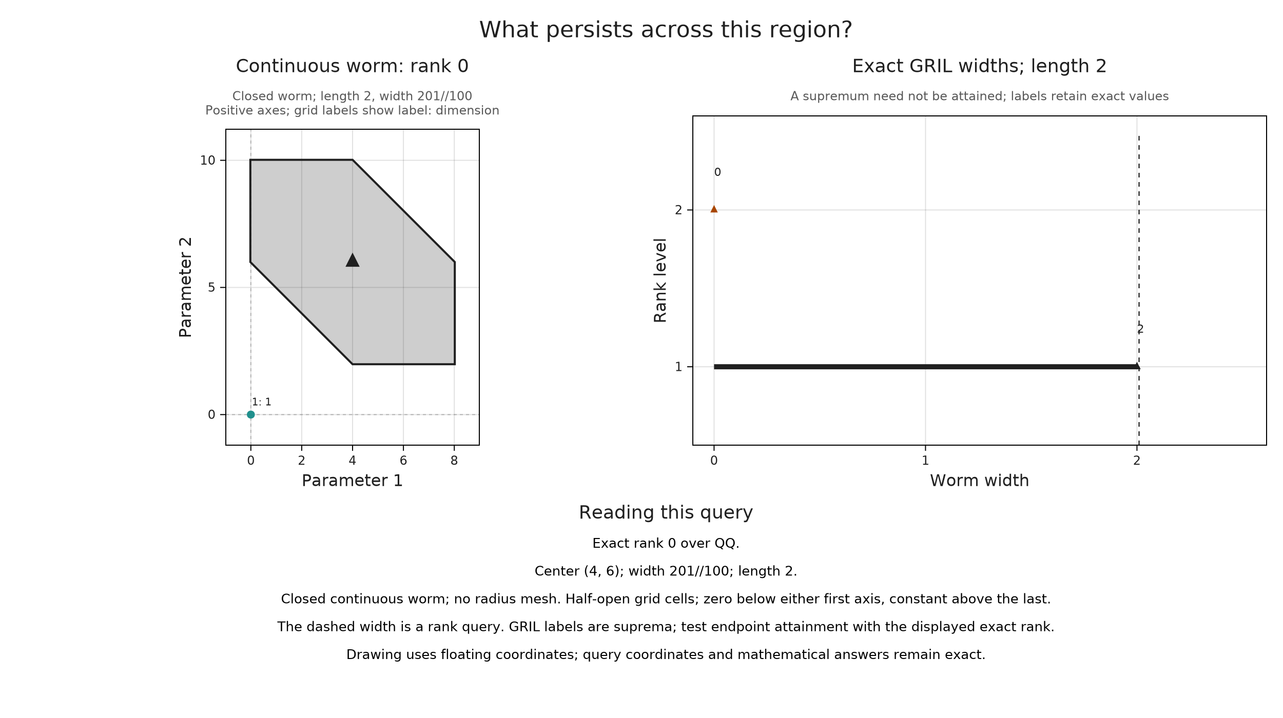
Try widths $3/2$, $2$ and $5/2$ in the prepared worm view. The center stays at $(4,6)$ and the length stays at two. The first worm lies inside the quadrant, the second touches its included boundary, and the third crosses into the zero extension. Their ranks are therefore one, one and zero. The level one supremum remains two throughout: the selected width tests a particular region, while the landscape records the boundary of all admissible widths.
Explore widths around the quadrant boundary
The selected width now crosses into the zero extension and the rank becomes zero. The landscape remains the same because changing the displayed width does not change its supremum. Selecting a retained level only redraws that result; moving the center requires new queries.
Arrays of landscape values use the order (center, level, length). A.feature_vector flattens them with center varying fastest. The next calculation chooses three centers explicitly, without assigning values between those centers.
probes = OP.gril(quadrant; centers=[(2, 5), (4, 6), (6, 3)], levels=(1, 2), lengths=(1, 2))
@assert A.gril_values(probes)[:, 1, 2] == QQ[1, 2, 3//2]
OP.visualize(probes; center=2, level=1, length=2)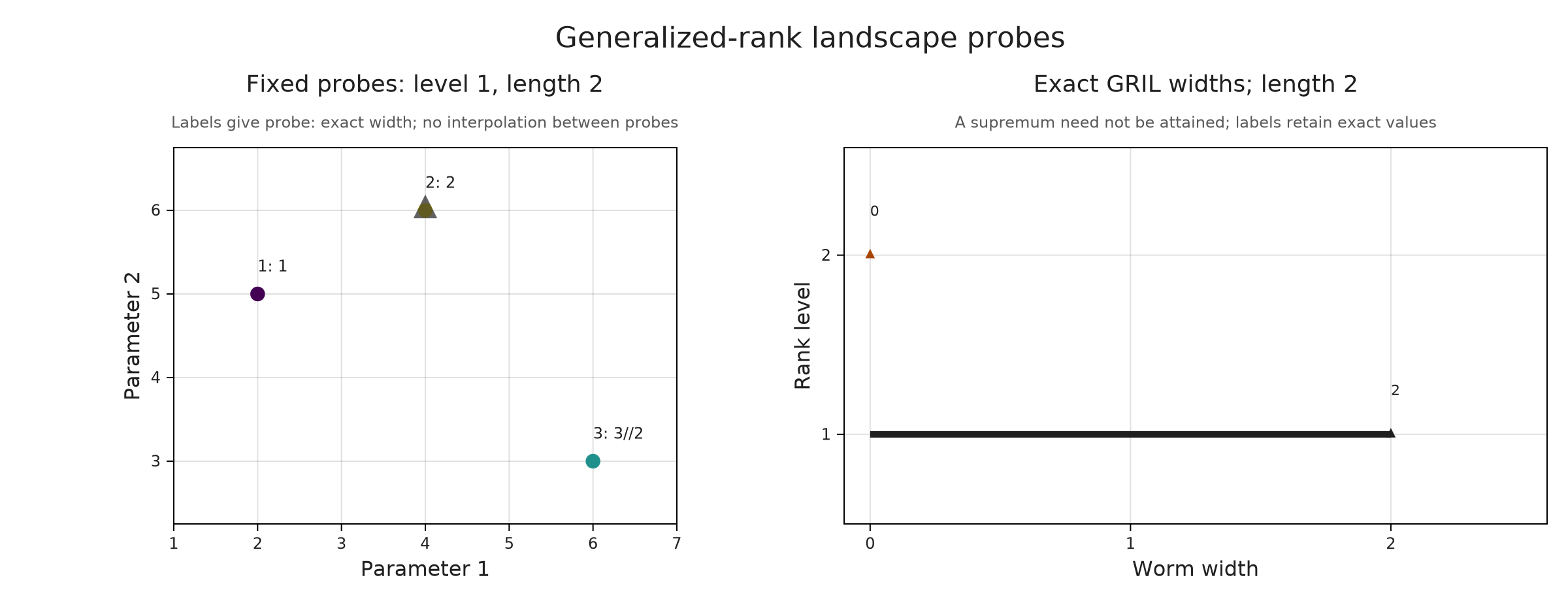
Optional: explore the same queries live
With WGLMakie installed and Julia running, the following calls open controls for the sessions we have already used:
using WGLMakie
OP.visualize(boundary_session; backend=:wglmakie)
OP.visualize(worm_session; backend=:wglmakie)
You can select finite labels or boundary occurrences, or change a worm's center, width, length and rank level. Text coordinates such as 1/3 retain their exact rational values; pointer coordinates are approximate. Hovering reads the retained answer without computing new matrices, and an invalid request or an exceeded work budget leaves the last valid state visible.
The choice of domain still matters. The boundary barcode certifies a region of grid labels under its theorem, while the worm query uses the specified continuous extension. The prepared browser comparisons above choose among already computed answers. These live controls require Julia because they can ask new queries.
Save a static view
Optional: save a static view
save_visual chooses a static export through the loaded renderer. Cosmetic styling stays separate from the query.
style = OP.VisualStyle(; palette=:grayscale)
A.select_inspection!(worm_session; width=2)
OP.visualize(A.inspection_snapshot(worm_session); style)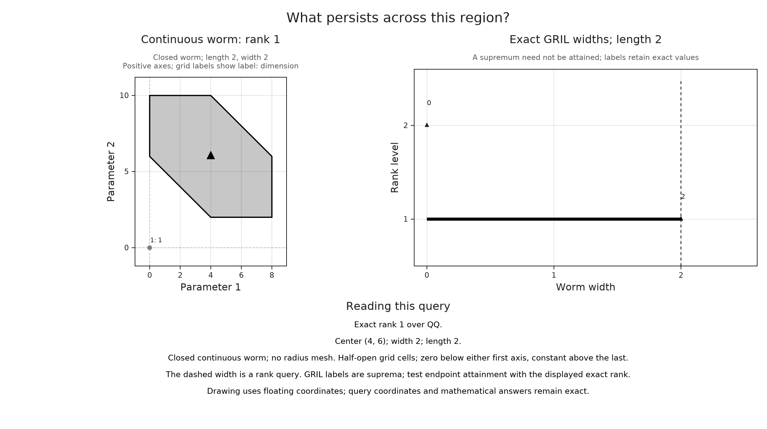
output_directory = mktempdir()
OP.save_visual(output_directory, "generalized-rank", A.inspection_snapshot(worm_session); style);
Prepare the region comparisons
Optional: Prepare the region comparisons
These cells save the fork and worm comparisons. The fork views use the same two modules as the opening example. The worm views hold the center and length fixed, checking the rank on either side of its known boundary. The compositions retain the mathematical drawings and matrices; the caption supplies their interpretation.
fork_views = (
    Symbol("Coincident images: both branches") => A.visual_spec(parallel;
        kind=:generalized_rank, vertices=1:3, witnesses=true),
    Symbol("Different images: both branches") => A.visual_spec(transverse;
        kind=:generalized_rank, vertices=1:3, witnesses=true),
    Symbol("Different images: second branch") => A.visual_spec(transverse;
        kind=:generalized_rank, vertices=[2,3], witnesses=true))
@assert Tuple(last(entry).metadata.rank for entry in fork_views) == (1, 0, 1)
mkpath(joinpath("tamerop_outputs", "regions"))
fork_pictures = Pair{Symbol,Any}[]
for (name, view) in fork_views
    picture = OP.compose_visuals((
        region=OP.visual_panel(view; panel=1),
        sections=OP.visual_panel(view; panel=2),
        quotient=OP.visual_panel(view; panel=3),
        comparison=OP.visual_panel(view; panel=4));
        columns=2, title=String(name),
        subtitle="Rational coefficients; generalized rank $(view.metadata.rank)")
    push!(fork_pictures, name => picture)
end
OP.save_visual_session(joinpath("tamerop_outputs", "regions", "fork.html"),
    (; fork_pictures...); title="Follow one branch or both",
    caption="The two modules have rational coefficients and the same separate arrow ranks. Change the selected region to compare agreement across both image lines with persistence along one branch. The diagrams show order relations, not physical coordinates.", size=(1200,900));
worm_views = Pair{Symbol,Any}[]
for (width, expected_rank, name) in ((3//2, 1, "Width 3/2: inside"),
        (2//1, 1, "Width 2: boundary included"),
        (5//2, 0, "Width 5/2: beyond the boundary"))
    A.select_inspection!(worm_session; width, length=2, level=1)
    @assert A.inspection_summary(worm_session).rank == expected_rank
    snapshot = A.inspection_snapshot(worm_session)
    picture = OP.compose_visuals((
        region=OP.visual_panel(snapshot; panel=1, limits=(x=(-2,10), y=(-1,12))),
        landscape=OP.visual_panel(snapshot; panel=2));
        columns=2, title=name,
        subtitle="Center (4,6); length 2; rank $expected_rank; level one supremum 2")
    push!(worm_views, Symbol(name) => picture)
end
@assert A.gril_values(landscape)[1,1,2] == 2
OP.save_visual_session(joinpath("tamerop_outputs", "regions", "worm_widths.html"),
    (; worm_views...); selected=Symbol("Width 2: boundary included"),
    title="When does the worm leave the quadrant?",
    caption="The rational quadrant module has dimension one on [0,∞)² and zero elsewhere. All views use center (4,6), length two and rank level one. Width two touches the included boundary; a larger width has generalized rank zero. The axes stay fixed as the width changes.", size=(1200,580));
The fork shows why maps with the same separate ranks can behave differently when we follow them together. The grid and worm examples then give two ways to choose the region of that question, with different geometric hypotheses. The branching region recipe is a compact starting point for your own finite module. For the constraint matrices and the exact search over widths, continue with Computing generalized rank and GRIL.
A.close_inspection!(boundary_session)
A.close_inspection!(worm_session);