Change of poset, refinement and Kan extensions
Changing a finite encoding means deciding how its old labels relate to the new ones, and then following the spaces and linear maps through that relation. An order map supplies the first part. Restriction and Kan extension use it to construct a module on the new base, while comparison morphisms describe how the old and new modules are related.
This account follows those constructions from their finite data to the matrices used in a comparison. The usage notebook explores two descriptions of a square; the reference gives the complete calling conventions. The category lesson explains which conclusions survive a change of base and which need further hypotheses.
The finite base is retained, not inferred from a drawing
An EncodingMap stores a source poset $Q$, a target poset $P$ and the target label $\pi(q)$ of every source vertex. Monotonicity means that $\pi(q)\leq\pi(q')$ whenever $q\leq q'$. The check uses the labelled orders; numeric labels and positions in a drawing do not determine those orders. A Hasse layout is a schematic of the cover relations, with no intermediate vertex between their endpoints.
A PModule stores the coefficient field, stalk dimensions and cover matrices. Its composition laws require different cover paths with the same endpoints to give the same map. Matrices have source columns and target rows throughout. Restriction along $\pi$ assigns $M(\pi(q))$ to $q$ and $M(\pi(q)\leq\pi(q'))$ to an ordered pair. A source cover can map to a longer chain in the target, requiring composition, or to an equality, requiring an identity matrix. This includes the empty identity at a zero stalk. Copying only target cover keys would therefore miss valid restricted maps.
The comparison viewer puts both branches on a declared common base before inspecting their maps. For a refinement it uses the two projections. For a single map $Q\to P$, it uses the identity on $Q$ and $\pi$, so both displayed modules live on $Q$. Geometry may help explain the labels, but the order maps determine the algebra.
Realized pairs and the product answer different questions
Suppose two finite classifiers $a:S\to P$ and $b:S\to R$ share the same labelled source. Their joint image is
\[J=\{(a(s),b(s)):s\in S\}\subseteq P\times R.\]
joint_encoding collects these pairs, removes duplicates, labels them in lexicographic order and gives them the order induced from the product. It returns the surjection $S\to J$ together with the projections to $P$ and $R$. Checking this result verifies surjectivity, distinct pairs, monotonicity and the induced order. Pair collection is linear in the finite source before sorting; storing and checking the explicit relation uses quadratic space and time in the number of distinct pairs, in addition to the order query costs.
A common refinement supplied with this result restricts both modules to $J$. Without it, different finite bases lead to an abstract product and restrictions on the entire product. Specialized product computations can reuse repeated blocks, but they preserve that meaning. Neither construction silently intersects continuous classifier fibers. Establishing which pairs occur over an infinite parameter space requires more information than a finite sample.
The pair panel reflects the distinction. Outlines mark pairs that belong to the actual comparison base; a supplied finite witness determines which pairs occur on its source. If the optional Cartesian background exceeds its display budget, it is omitted with a notice while the actual common pairs remain. An absent drawing cell does not assert that a stalk is zero.
Kan extensions retain chosen limit and colimit coordinates
For a module $M:Q\to\mathrm{Vect}_k$ over a field $k$ and an order map $\pi:Q\to P$, the left Kan stalk at $p$ is the colimit over $I_p=\{q:\pi(q)\leq p\}$. A colimit combines all these spaces while identifying a vector with its image along every arrow. The right Kan stalk is the limit over $J_p=\{q:p\leq\pi(q)\}$. Its vectors are families whose entries agree under the diagram's maps. These pointwise formulas come from the categorical theory of Kan extensions and adjunctions; the finite matrices described below are TamerOp's implementation of them.
Quotient coordinates for the left Kan extension
Let $S=\bigoplus_{q\in I_p}M(q)$. For an arrow $u\leq v$ and a vector $x\in M(u)$, place $x$ in the $u$ summand and $-M(u\leq v)x$ in the $v$ summand. These relation vectors span the subspace to be identified with zero. If Rel has these vectors as columns, the colimit is $S/\operatorname{im}(\mathrm{Rel})$. Cover relations suffice because longer relations follow by composition.
The implementation assembles the transpose of this relation matrix and computes a nullspace basis N. Put Q = transpose(N), using Q here for a matrix rather than the source poset. Then Q*Rel=0, and the nullspace dimension shows that ker(Q)=im(Rel). Thus Q is a quotient coordinate map: two vectors of S have the same Q coordinates precisely when their difference is a relation.
To choose representatives, take a left inverse J of N, so J*N=I, and put W = transpose(J). The equality Q*W=I says that W is a section: it selects a vector in S for each quotient coordinate. In the rational elimination route, the identity block on free rows of the nullspace basis supplies this left inverse by row selection. Other field routes use the corresponding field linear algebra. These equalities describe the exact field calculation; RealField uses its declared tolerances for nullspaces and coordinate solves, as explained in numerical algebra.
A diagram map F that preserves relations induces the quotient matrix Q_target * F * W_source. This follows a quotient vector to its chosen representative, applies F, and then takes target quotient coordinates. A different section changes the representative only by a source relation, whose image is a target relation killed by Q_target; the induced map is therefore independent of that section. The quotient bases themselves remain choices, so their coordinate matrices need not look identical after a separate construction.
Consider the poset with $1<2$ and $1<3$, collapsed to one point. The module $M=(0,k,k)$ has no nonzero relation vectors, giving colimit $k^2$. The constant module $N=(k,k,k)$ has relations $e_1-e_2$ and $e_1-e_3$, giving colimit $k$. Here $e_i$ denotes the vector from the copy of $k$ at vertex $i$.
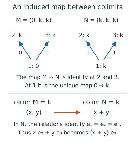
This schematic follows the map from $M$ to $N$ that is identity at vertices 2 and 3. In the target colimit, the classes of $e_2$ and $e_3$ agree, so $(x,y)$ maps to $x+y$. Knowing only the dimensions would leave this matrix undetermined. Arrows within each module carry their scalar maps, and the vertex labels are the same in both diagrams.
For these coordinates, Q_target=[1 1 1], and F includes the two source summands as the last two target summands. Their product is [1 1], the addition map. This example also explains why a nullspace inclusion N must not be mistaken for a quotient section. The required equation is Q*W=I; transpose(N)*N need not be invertible over a general field.
Kernel coordinates for the right Kan extension
For $J_p$, form the finite product of its stalks, represented as a direct sum because the index set is finite. A family $(x_q)$ belongs to the limit when $x_v-M(u\leq v)x_u=0$ for every cover $u\leq v$ in this set. The corresponding constraint matrix C therefore gives the limit as ker(C).
A basis matrix K includes limit coordinates into the family of stalk coordinates. Its left inverse L recovers coordinates from a compatible family, with L*K=I. For $p\leq p'$, the index set $J_{p'}$ is contained in $J_p$, so projecting a compatible family to the smaller set and applying the new left inverse gives the target structure map. Left Kan maps similarly come from inclusions $I_p\subseteq I_{p'}$, followed by quotient coordinates. The stored coordinate maps supply the units and counits and the induced maps of module morphisms.
When one stalk already determines the result
If $I_p$ has a maximum $q_{\max}$, every summand maps to $M(q_{\max})$ and these maps describe its colimit. TamerOp then uses that stalk directly, with its structure maps forming the quotient map and its summand inclusion forming a section. No general relation nullspace is needed. Dually, a minimum in $J_p$ determines the limit; its outgoing maps produce the compatible family, and projection back to that stalk recovers its coordinates. An empty indexing set gives a zero dimensional result in either case.
The preparation records index sets, cover edges, coordinate offsets and how neighboring sets include into one another. General fibers require field linear algebra on their sparse relation or constraint matrices; costs depend on the sum of their stalk dimensions and the size and sparsity of these equations. Fibers can be computed independently with threading enabled. The retained preparation and intermediate coordinates can be reused through the session cache, while the viewer receives an already computed Kan object. It does not construct a Kan extension or a missing comparison as part of drawing.
What a commuting-square certificate actually checks
Let $L,R$ be the modules restricted to the common base, and suppose a supplied comparison has components $f_q:L(q)\to R(q)$. For a selected ordered pair, the viewer computes both sides of
\[R(q\leq q')f_q=f_{q'}L(q\leq q').\]
Each side carries a vector from $L(q)$ to $R(q')$. The four matrices and two products are retained in the readout. Once the input modules satisfy their path relations, checking this equation on every cover proves it on every ordered pair by composition. A natural morphism is an isomorphism precisely when every component is invertible, so the additional component ranks determine the finite natural isomorphism result. A comparison in the opposite direction exchanges $L$ and $R$.
The prepared square comparison changes the selected pair while retaining the identity comparison between two descriptions of a square. It displays both products for comparable pairs and the order obstruction when there is no forward square.
Matrices of the wrong shape or belonging to incompatible endpoints are rejected. A comparison with suitable shapes but failed naturality equations can be drawn with those failures visible. Reversed or incomparable pairs have no forward square. Real coefficient comparisons report their residuals and tolerances, with ranks determined by the numerical field policy. Exact matrices and the selected products are copied into the snapshot, so later cache activity does not change its saved equations.
These checks concern the displayed finite representation category. For example, the constant module on the four element poset with two minima below two maxima has an invertible left Kan unit for collapse to one point. Its degree one self-Ext nevertheless differs from that of the resulting vector space. The category lesson derives this counterexample; the comparison result retains finite_poset_representations and does not assert ambient or derived invariance when its component checks pass.
Preparation, navigation and optimization boundaries
Inspection preparation validates the order maps, supplied modules, agreement of the restrictions on covers and any comparison. It computes deterministic Hasse layouts and supported planar classifier geometry. Supplying a lazy encoding for these checks materializes its finite module because dimensions alone cannot determine the equations being checked.
A session retains this preparation. A selection requests only its maps and products, although obtaining a transitive map can still require composition. Selecting a side label retains all its preimages; selecting a parameter classifies it independently through both retained classifiers. Hover reads stored geometry and IDs. None of these operations chooses an arbitrary representative or infers ambient order from finite labels.
An update constructs and validates its proposed state before replacing the current state, so a failure preserves the old snapshot and revision. Closing releases prepared inputs and listeners while keeping the final snapshot. The inspection account develops this lifecycle for the shared session interface. Any reuse must preserve the bases, comparison maps, coefficient policy, finite witness and stated display limits, since these data determine what the inspected equations mean.
See the implementation bibliography.